
Overview
insight.cast builds infectious disease forecasts in a
few steps:
-
get_data()orcheck_data()fetches or validates surveillance data. -
get_ncast()optionally corrects recent weeks for reporting delays. -
get_cv()optionally compares models by time-series cross-validation. -
get_fcast()produces a forecast and ensemble.
See Planning an infectious disease forecast before starting a new forecasting project.
Step 1: Get data
Fetch weekly influenza hospital admissions for New York and
California from the CDC
NHSN through epidatr.
Set revisions = TRUE to fetch the history needed for
nowcasting.
# You may need a Delphi API key to run this code.
# See `?epidatr::get_api_key()` for details.
df <- get_data(pathogen = "flu", geo_value = c("ny", "ca"), revisions = TRUE)
Pass other data through check_data(). See
vignette("external_data") for the required format.
tail(example_data)
#> # A tibble: 6 × 5
#>   as_of      location target          target_end_date observation
#>   <date>     <chr>    <chr>           <date>                <dbl>
#> 1 2025-12-07 CA       wk inc flu hosp 2025-12-06              233
#> 2 2025-12-14 CA       wk inc flu hosp 2025-12-06              259
#> 3 2025-12-07 NY       wk inc flu hosp 2025-12-06             1160
#> 4 2025-12-14 NY       wk inc flu hosp 2025-12-06             1171
#> 5 2025-12-14 CA       wk inc flu hosp 2025-12-13              412
#> 6 2025-12-14 NY       wk inc flu hosp 2025-12-13             1462
df <- check_data(example_data)
autoplot(df)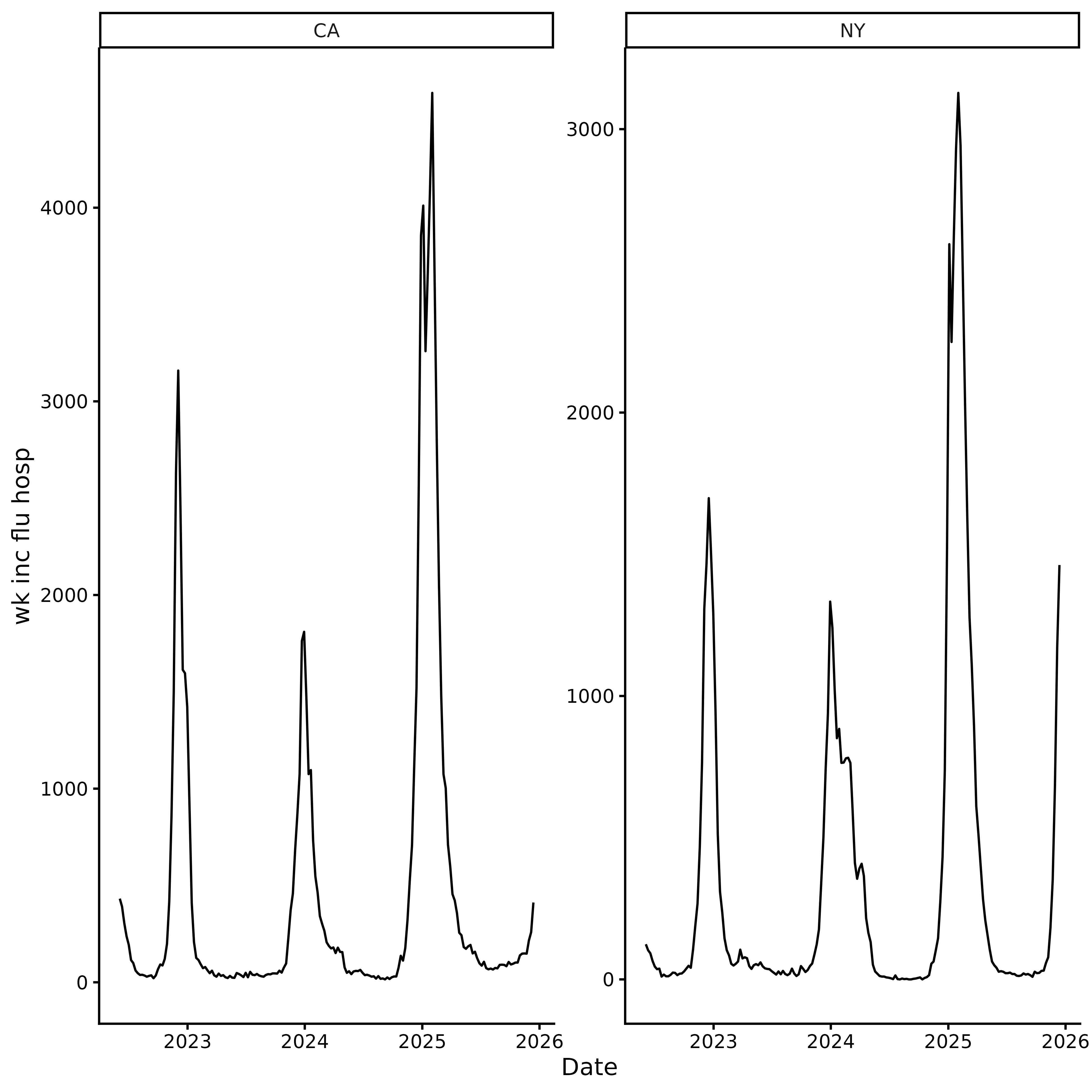
Step 2: Nowcast (optional)
Recent surveillance counts may be incomplete because reports arrive late. Using them directly can bias forecasts downwards.
get_ncast() estimates their final values. By default it
corrects the last two weeks and leaves earlier observations
unchanged.
ncast <- get_ncast(df)
ncast
#> <insightcast_ncast>
#> Target:   wk inc flu hosp
#> Series:   2 (location)
#> Window:   2022-06-04 to 2025-12-13 (7-day interval)
#> Nowcast:  2025-12-06 to 2025-12-13
autoplot(ncast)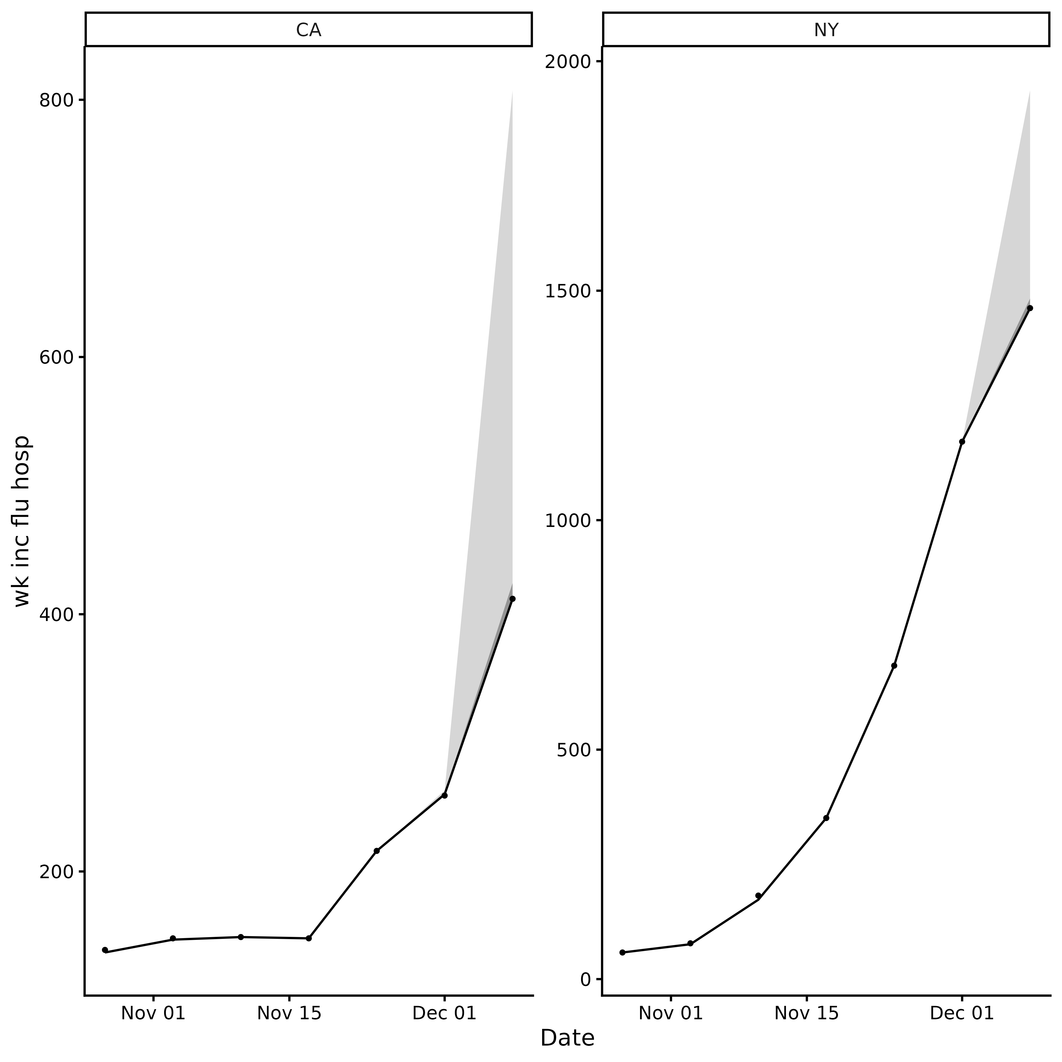
For corrected weeks, ncast$data contains
ncast_lower and ncast_upper 95% credible
interval bounds. get_fcast() carries this uncertainty into
the forecast.
Step 3: Forecasting
The forecast workflow has two steps:
-
get_cv()evaluates models and ranks them by weighted interval score (WIS). -
get_fcast()fits the models to all available data, combines the besttop_nand forecastshreporting intervals ahead.
The default models are:
| Model | Description |
|---|---|
NAIVE |
Carries the latest value forwards |
ETS |
Exponential smoothing |
THETA |
Theta method |
ARIMA |
Automatically selected ARIMA model |
Cross-validation
get_cv() performs rolling-origin time series
cross-validation.
Three arguments set the evaluation period:
h: forecast horizon in reporting intervals.-
step: spacing between forecast origins.-
step = h(default) produces non-overlapping forecasts and is the fastest option. -
step < hproduces more, overlapping forecasts.
-
-
Supply one origin argument:
-
n_origins: the number of forecast origins. -
eval_start_date: the date of the first forecast origin. -
origins: explicit dates, including non-contiguous dates.
-
A forecast origin at time d predicts intervals
d to d + h - 1, so n_origins
origins spaced step intervals apart cover the last
h + (n_origins - 1) * step reporting intervals of the
series. For example, with h = 4, step = 4, and
n_origins = 3, the evaluation period covers the last 12
intervals:
Forecast 1: [d,   d+1, d+2,  d+3]
Forecast 2: [d+4, d+5, d+6,  d+7]
Forecast 3: [d+8, d+9, d+10, d+11]
More origins give a broader comparison but leave less data before the first model fit.
The result contains forecasts and scores for each model and series.
cv <- get_cv(ncast, h = 4, n_origins = 16)
cv
#> <insightcast_cv>
#> Target:   wk inc flu hosp
#> Series:   2 (location)
#> Window:   2022-06-04 to 2025-12-13 (7-day interval)
#> CV:       4 models x 16 origins (h = 4)
Plot relative WIS by model and series. Values below 1 are better than average.
autoplot(cv)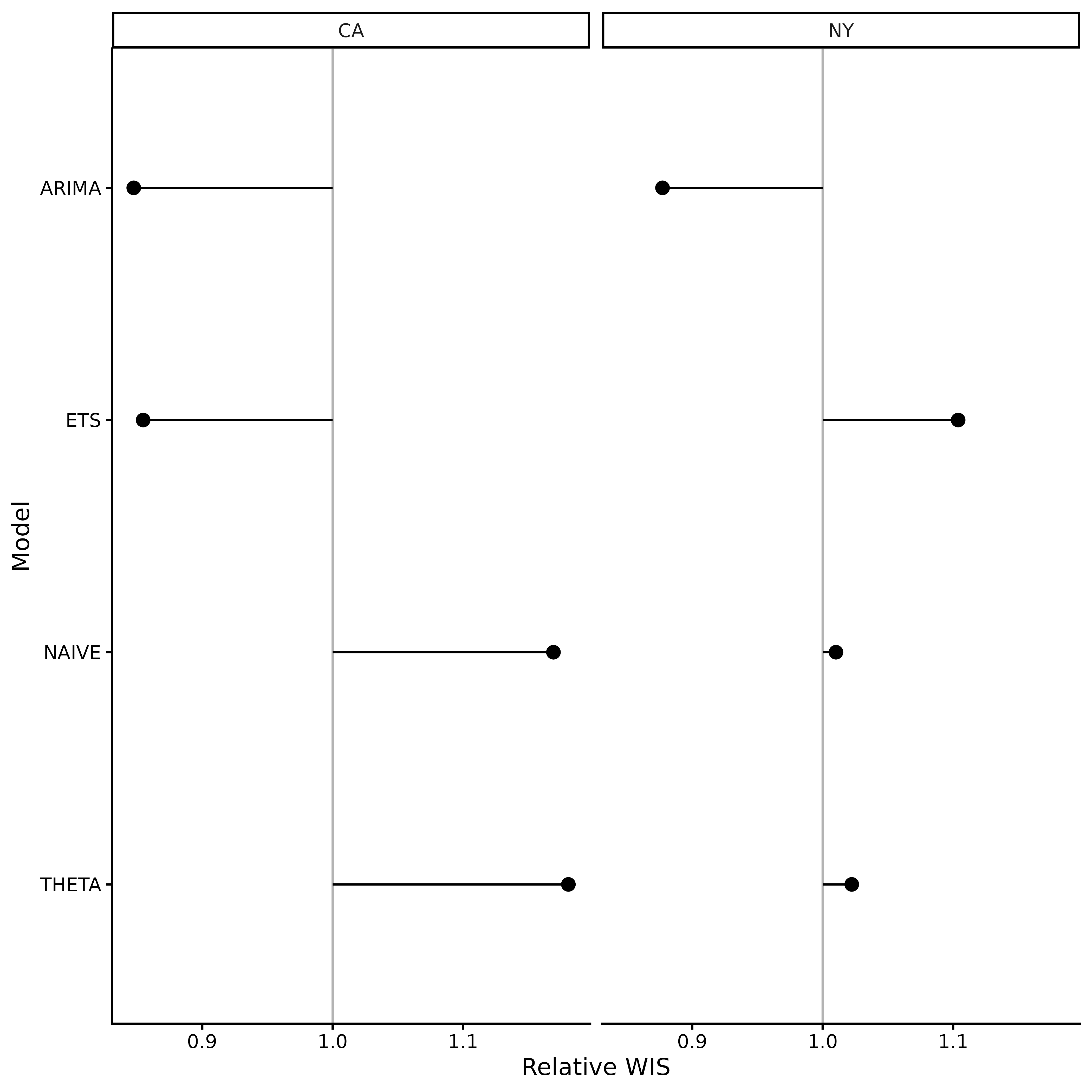
Forecast
get_fcast() combines the best top_n models.
Its horizon defaults to the value used by get_cv().
fcast <- get_fcast(cv, top_n = 2)
fcast
#> <insightcast_fcast>
#> Target:   wk inc flu hosp
#> Series:   2 (location)
#> Forecast: 2025-12-20 to 2026-01-10 (h = 4)
#> Models:   4 + ENSEMBLE
Plot the ensemble, or set model to inspect one
model:
autoplot(fcast)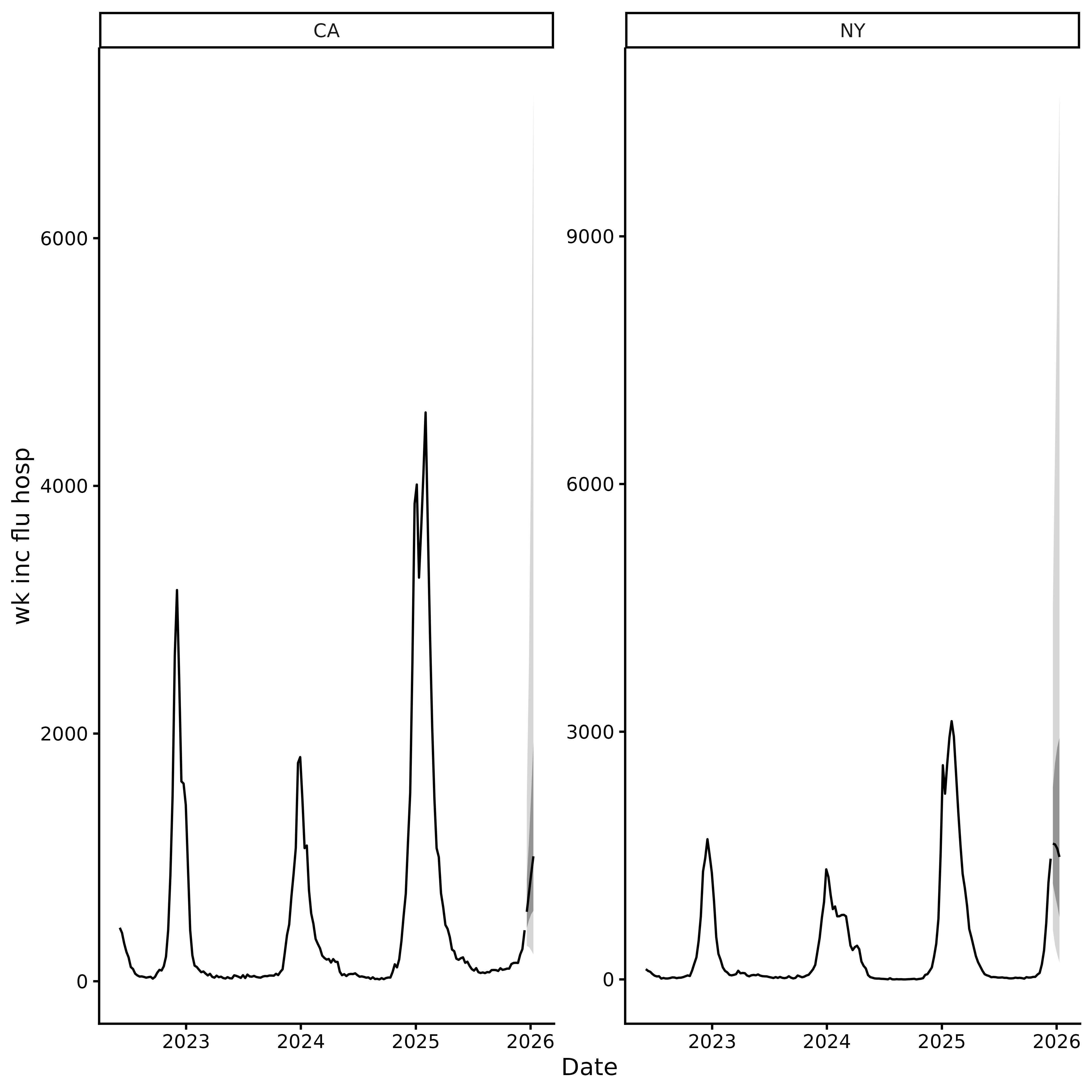
Adding custom models
Pass any fable model through
models. insight.cast.odin
adds transmission models built with odin2. Combine custom
specifications with default_models() to retain the
defaults:
library(fable)
library(fable.prophet)
library(EpiEstim)
library(projections)
library(insight.cast.odin)

# Illustrative inputs for the joint HHH4 models. Replace the connections with
# ones appropriate to your application; rows are sources and columns recipients.
adjacency <- rbind(
  CA = c(CA = 0, NY = 1),
  NY = c(CA = 1, NY = 0)
)
population <- c(CA = 39.4e6, NY = 20.0e6)
population <- population / sum(population)
annual_seasonality <- surveillance::addSeason2formula(
  f = ~1,
  S = 1,
  period = round(365.25 / ncast$interval)
)

my_models <- c(
  default_models(),
  list(
    # Statistical models
    CUSTOM_ARIMA = ARIMA(observation ~ pdq(1, 1, 0)),

    # Epidemiological models
    EPIESTIM = EPIESTIM(
      observation,
      mean_si = 3.5,
      std_si = 2.1,
      rt_window = ncast$interval
    ),
    ODIN2_SIR = odin_sir(observation),
    ODIN2_SEIR = odin_seir(observation),
    HHH4_AR_END = HHH4(
      observation,
      control = list(
        ar = list(f = ~1, lag = 1),
        ne = list(f = ~ -1),
        end = list(f = annual_seasonality),
        family = "NegBin1"
      ),
      population = population
    ),
    HHH4_FULL = HHH4(
      observation,
      control = list(
        ar = list(f = ~1, lag = 1),
        ne = list(f = ~1, lag = 1, normalize = TRUE),
        end = list(f = annual_seasonality),
        family = "NegBin1"
      ),
      neighbourhood = adjacency,
      population = population
    ),

    # Machine learning models
    PROPHET = prophet(observation ~ season("year")),
    NNETAR = NNETAR(observation),

    # Foundation models
    CHRONOS = FOUNDATION(log(observation), "chronos"),
    TIMESFM = FOUNDATION(log(observation), "timesfm")
  )
)

cv <- get_cv(
  ncast,
  n_origins = 16,
  models = my_models
)

fcast <- get_fcast(cv, top_n = 3)
Export to RespiLens
Save the Hubverse output as a CSV, then upload it to myRespiLens:
write.csv(fcast$hub$model_out_tbl, "respilens.csv", row.names = FALSE)