Forecasting connected time series with HHH4 • insight.cast

Overview

Most insight.cast models fit each series separately. HHH4 fits them jointly, so recent counts in one series can help predict another.

A unit is one key value, such as a state when key = "location". HHH4 requires one key column and a meaningful set of connected units.

Model components

HHH4 models the expected count as the sum of three components:

$\text{expected count} = \text{endemic} + \text{autoregressive} + \text{neighbour}.$

Component	Uses
Endemic (`end`)	Background incidence, population, and seasonality
Autoregressive (`ar`)	Previous counts in the same unit
Neighbour (`ne`)	Previous counts in connected units

The example below uses these settings:

Setting	Meaning
`f = ~1`	Turn a component on with one effect shared across units
`f = ~-1`	Turn a component off
`lag = 1`	Use counts from the previous reporting period
`S = 1`	Use one smooth annual rise and decline
`family = "NegBin1"`	Allow extra count variability, shared across units
`normalize = TRUE`	Rescale each source row of the neighbour matrix to sum to one

S = 1 is one seasonal harmonic: a sine/cosine pair that learns the timing and size of a repeating annual cycle.

Example

This example forecasts weekly influenza hospital admissions in Connecticut, New Jersey, New York and Pennsylvania. The vignette loads objects fitted to data available on 8 August 2026. Data collection and model fitting remain disabled; the saved plots are rebuilt with the article.

Data

# install.packages("surveillance") # Run once if needed.
library(insight.cast)
library(surveillance)

states <- c("ct", "nj", "ny", "pa")
flu <- get_data(pathogen = "flu", geo_value = states)

flu
#> <insightcast_data>
#> Target:   wk inc flu hosp
#> Series:   4 (location)
#> Window:   2020-08-08 to 2026-08-08 (7-day interval)
autoplot(flu)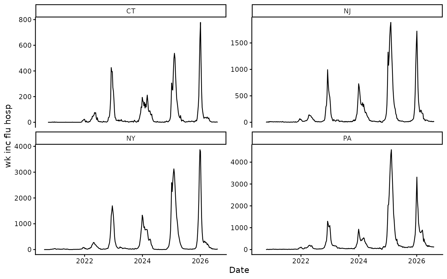

Weekly influenza hospital admissions by state.

HHH4 needs one count target, one series key, and aligned reporting dates. For external data, use check_data(data, key = "location").

Connections and population

Rows of the connection matrix are sources and columns are receiving units. Here, 1 means that two states share a border.

adjacency <- rbind(
  CT = c(CT = 0, NJ = 0, NY = 1, PA = 0),
  NJ = c(CT = 0, NJ = 0, NY = 1, PA = 1),
  NY = c(CT = 1, NJ = 1, NY = 0, PA = 1),
  PA = c(CT = 0, NJ = 1, NY = 1, PA = 0)
)

population <- c(
  CT = 3.6e6,
  NJ = 9.5e6,
  NY = 20.0e6,
  PA = 13.0e6
)
population <- population / sum(population)

Population is used as an offset, allowing larger states to have a larger background count. All names must match the series key values exactly.

Model specifications

First define one annual cycle for the endemic component:

annual_seasonality <- addSeason2formula(
  f = ~1,
  S = 1,
  period = round(365.25 / flu$interval)
)

Compare four component structures:

Model	Endemic	Autoregressive	Neighbour
`HHH4_END`	on	off	off
`HHH4_AR_END`	on	on	off
`HHH4_NE_END`	on	off	on
`HHH4_FULL`	on	on	on

end_control <- list(
  ar = list(f = ~ -1),
  ne = list(f = ~ -1),
  end = list(f = annual_seasonality),
  family = "NegBin1"
)

ar_end_control <- end_control
ar_end_control$ar <- list(f = ~1, lag = 1)

ne_end_control <- end_control
ne_end_control$ne <- list(f = ~1, lag = 1, normalize = TRUE)

full_control <- ar_end_control
full_control$ne <- ne_end_control$ne

Create the model specifications:

hhh4_models <- list(
  HHH4_END = HHH4(
    observation,
    control = end_control,
    population = population
  ),
  HHH4_AR_END = HHH4(
    observation,
    control = ar_end_control,
    population = population
  ),
  HHH4_NE_END = HHH4(
    observation,
    control = ne_end_control,
    neighbourhood = adjacency,
    population = population
  ),
  HHH4_FULL = HHH4(
    observation,
    control = full_control,
    neighbourhood = adjacency,
    population = population
  )
)

Compare and forecast

Compare the HHH4 specifications with the default insight.cast models using the same forecast origins:

models <- c(default_models(), hhh4_models)

set.seed(2026)
cv <- get_cv(
  flu,
  h = 4,
  n_origins = 12,
  models = models
)

cv
#> <insightcast_cv>
#> Target:   wk inc flu hosp
#> Series:   4 (location)
#> Window:   2020-08-08 to 2026-08-08 (7-day interval)
#> CV:       8 models x 12 origins (h = 4)
autoplot(cv)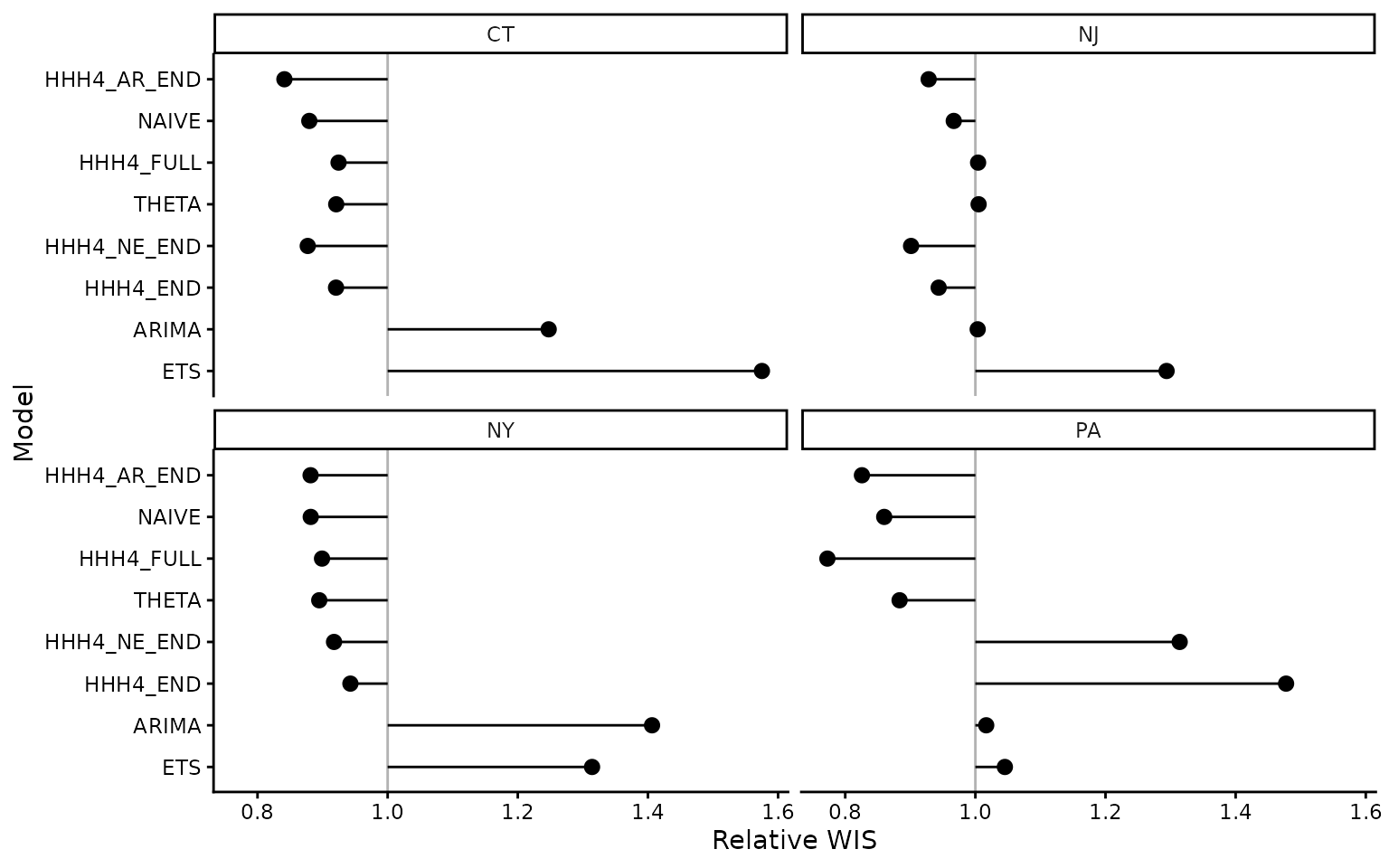

Cross-validation performance by model and state.

Passing hhh4_models to get_fcast() refits all four specifications. The default plot shows their ensemble; set model to inspect one specification.

set.seed(2026)
fcast <- get_fcast(cv, models = hhh4_models)

fcast
#> <insightcast_fcast>
#> Target:   wk inc flu hosp
#> Series:   4 (location)
#> Forecast: 2026-08-15 to 2026-09-05 (h = 4)
#> Models:   4 + ENSEMBLE
autoplot(fcast)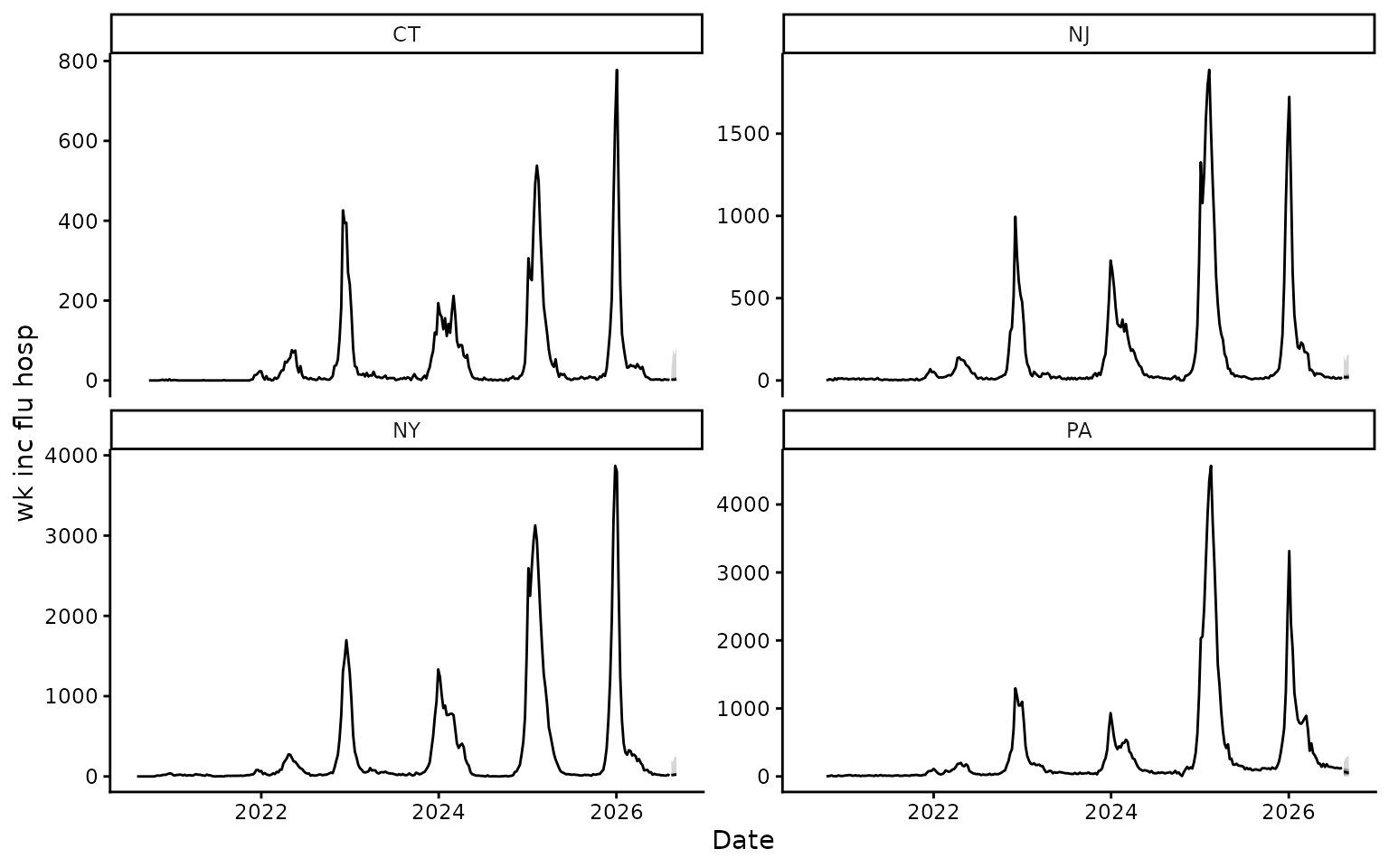

Ensemble forecast from the four HHH4 specifications.

autoplot(fcast, model = "HHH4_FULL")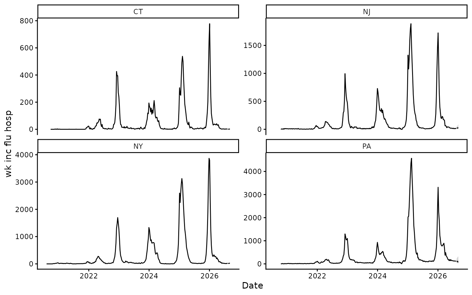

Forecast from the full endemic, autoregressive and neighbour model.

Add a covariate

Add a covariate to the component it affects and supply its values in control$data. For example, school holidays may affect the endemic component:

h <- 4L
dates <- seq(
  min(flu$data$target_end_date),
  max(flu$data$target_end_date) + h * flu$interval,
  by = flu$interval
)
school_holiday <- as.integer(format(dates, "%m") %in% c("07", "08"))

holiday_control <- full_control
holiday_control$end$f <- addSeason2formula(
  f = ~ 1 + school_holiday,
  S = 1,
  period = round(365.25 / flu$interval)
)
holiday_control$data <- list(school_holiday = school_holiday)

hhh4_models$HHH4_SCHOOL_HOLIDAY <- HHH4(
  observation,
  control = holiday_control,
  neighbourhood = adjacency,
  population = population
)

This example treats July and August as school holidays. Time-varying covariates must cover the observed history and forecast horizon. See ?surveillance::hhh4 for other controls.

Reference

Meyer S, Held L, Höhle M (2017). Spatio-temporal analysis of epidemic phenomena using the R package surveillance. Journal of Statistical Software 77(11), 1–55.