
Overview
In May 2026, the Democratic Republic of the Congo reported an Ebola outbreak caused by the Bundibugyo strain. By July, 2,423 cases and 967 deaths had been reported. This example forecasts incidence using surveillance data from the Institut National de Recherche Biomédicale.
The vignette loads precomputed data, cross-validation and forecast objects. Model-fitting chunks are disabled, but all plots are generated when the article is built.
Data
The example uses the six locations with the most confirmed cases. Missing days carry the previous cumulative count forwards, and downward revisions are removed. Leading zeros are dropped before log transformation.
library(dplyr)
library(tidyr)
library(ggplot2)

ebola <- read.csv(
  "https://raw.githubusercontent.com/scc-usc/ebola2026/refs/heads/main/hubverse_observed_data.csv"
) |>
  filter(
    target == "insp_sitrep__cumulative_confirmed_cases__daily",
    !is.na(location)
  ) |>
  mutate(target_end_date = as.Date(target_end_date))

top_locations <- ebola |>
  slice_max(target_end_date, by = location) |>
  slice_max(observation, n = 6) |>
  pull(location)

ebola <- ebola |>
  filter(location %in% top_locations) |>
  arrange(location, target_end_date) |>
  group_by(location) |>
  complete(
    target_end_date = seq(
      min(target_end_date),
      max(target_end_date),
      by = "day"
    )
  ) |>
  fill(observation, .direction = "down") |>
  mutate(observation = cummax(coalesce(observation, 0))) |>
  filter(cumsum(observation > 0) > 0) |>
  ungroup() |>
  mutate(target = "insp_sitrep__cumulative_confirmed_cases__daily")
insight.cast workflow
Validate the data
check_data() standardises the columns and returns an
insightcast_data object.
library(insight.cast)
data <- ebola |> check_data()
data
#> <insightcast_data>
#> Target:   insp_sitrep__cumulative_confirmed_cases__daily
#> Series:   6 (location)
#> Window:   2026-05-15 to 2026-07-26 (1-day interval)
data |> autoplot()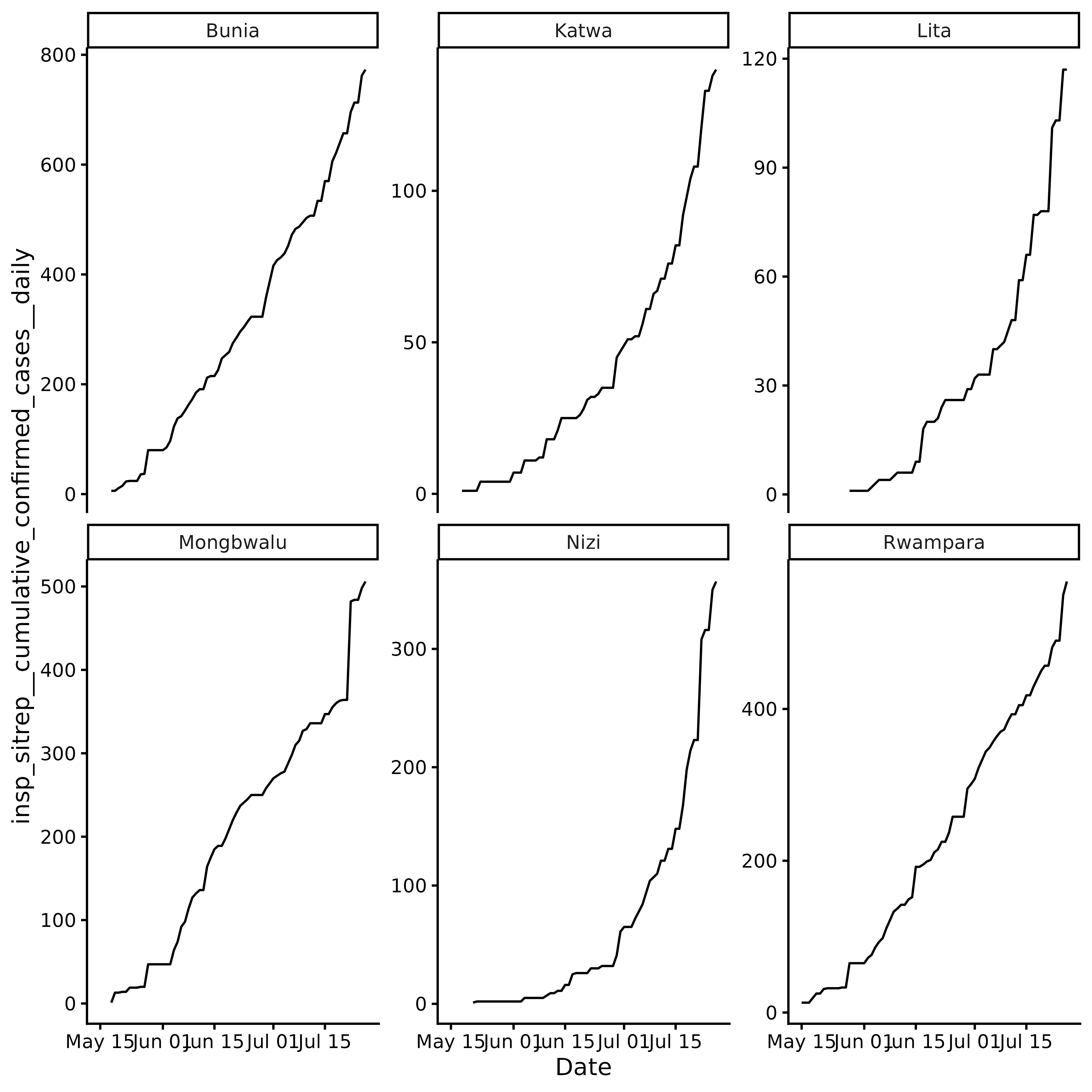
Daily cumulative confirmed cases by location.
Revision history is unavailable, so the workflow skips
get_ncast().
Cross-validation
Compare the default models with a custom ARIMA model, a neural network, Prophet and four foundation models:
library(fable)
library(fable.prophet)

models <- c(
  default_models(),
  list(
    CUSTOM_ARIMA = ARIMA(log(observation) ~ pdq(1, 1, 0)),
    NNETAR = NNETAR(log(observation), n_networks = 10),
    PROPHET = prophet(log(observation)),
    CHRONOS = FOUNDATION(log(observation), "chronos"),
    TIMESFM = FOUNDATION(log(observation), "timesfm"),
    SUNDIAL = FOUNDATION(log(observation), "sundial"),
    MOIRAI = FOUNDATION(log(observation), "moirai")
  )
)
Forecast seven days ahead from 16 daily origins. The evaluation covers 22 days.
cv <- data |>
  get_cv(
    h = 7,
    step = 1,
    n_origins = 16,
    models = models
  )
cv
#> <insightcast_cv>
#> Target:   insp_sitrep__cumulative_confirmed_cases__daily
#> Series:   6 (location)
#> Window:   2026-05-15 to 2026-07-26 (1-day interval)
#> CV:       11 models x 16 origins (h = 7)
cv |>
  autoplot() +
  ggplot2::scale_x_continuous(transform = "log2")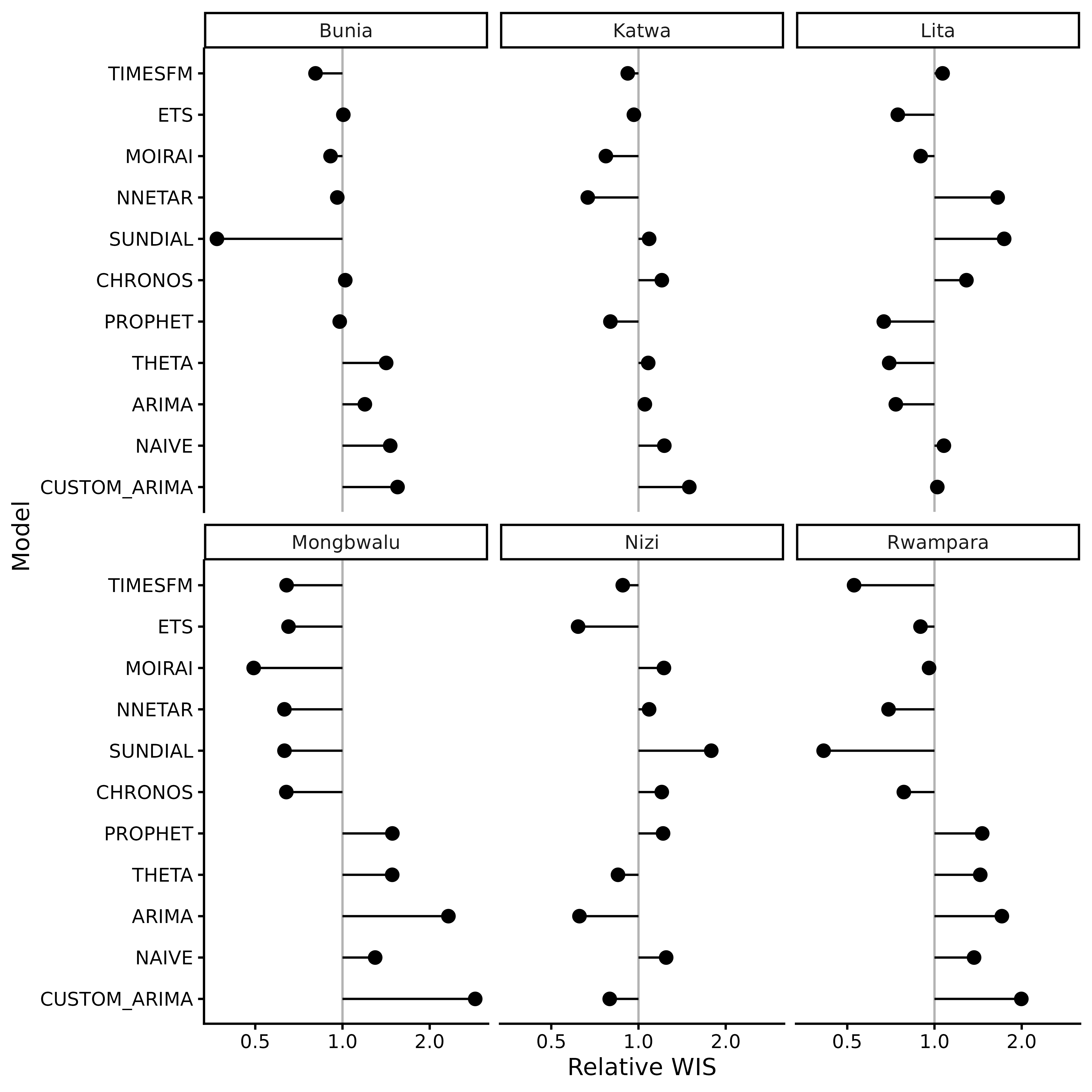
Cross-validation performance by model and location.
autoplot() shows relative WIS from
cv$score. Raw WIS depends on the scale of each series;
relative WIS supports comparison across locations. On the log scale, 0.5
and 2 are equally far from the reference value of 1.
Use cv$score for custom summaries, such as raw WIS by
model and location:
cv$score |>
  group_by(location) |>
  arrange(wis, .by_group = TRUE) |>
  mutate(model_id_ordered = paste(model_id, location, sep = "__")) |>
  ggplot(aes(y = reorder(model_id_ordered, wis), x = wis)) +
  facet_wrap(~location, scales = "free") +
  geom_col(aes(fill = model_id), show.legend = FALSE) +
  scale_y_discrete(labels = \(x) sub("__.*$", "", x)) +
  theme_classic() +
  labs(y = "Model", x = "WIS")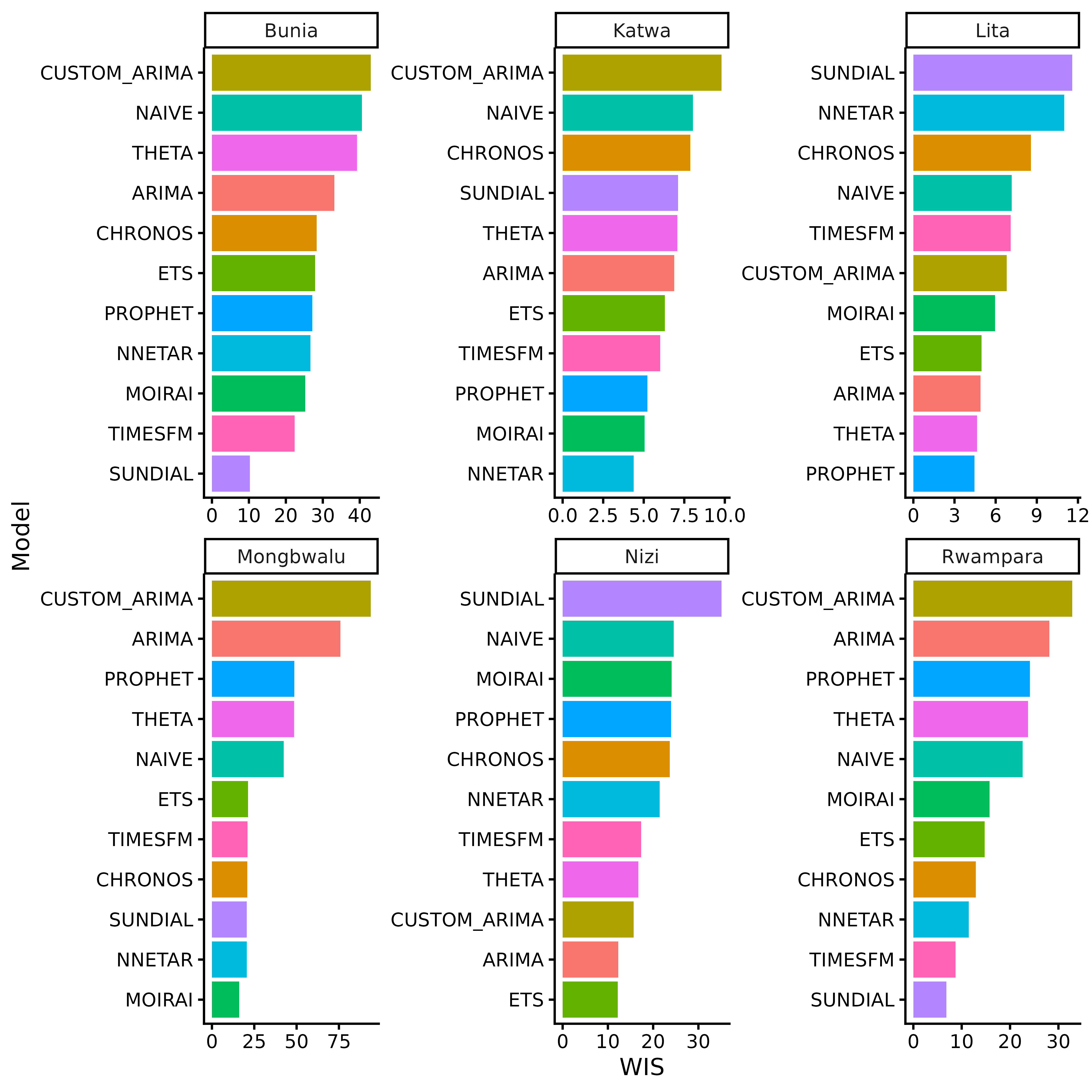
Forecasting
By default, get_fcast() combines the three best models
for each location.
fcast <- cv |> get_fcast()
fcast
#> <insightcast_fcast>
#> Target:   insp_sitrep__cumulative_confirmed_cases__daily
#> Series:   6 (location)
#> Forecast: 2026-07-27 to 2026-08-02 (h = 7)
#> Models:   9 + ENSEMBLE
fcast$meta$selection
#> # A tibble: 18 × 2
#>    location  model_id
#>    <chr>     <chr>
#>  1 Bunia     SUNDIAL
#>  2 Bunia     TIMESFM
#>  3 Bunia     MOIRAI
#>  4 Katwa     NNETAR
#>  5 Katwa     MOIRAI
#>  6 Katwa     PROPHET
#>  7 Lita      PROPHET
#>  8 Lita      THETA
#>  9 Lita      ARIMA
#> 10 Mongbwalu MOIRAI
#> 11 Mongbwalu NNETAR
#> 12 Mongbwalu SUNDIAL
#> 13 Nizi      ETS
#> 14 Nizi      ARIMA
#> 15 Nizi      CUSTOM_ARIMA
#> 16 Rwampara  SUNDIAL
#> 17 Rwampara  TIMESFM
#> 18 Rwampara  NNETAR
autoplot() shows the median and 50% and 95% prediction
intervals.
fcast |> autoplot()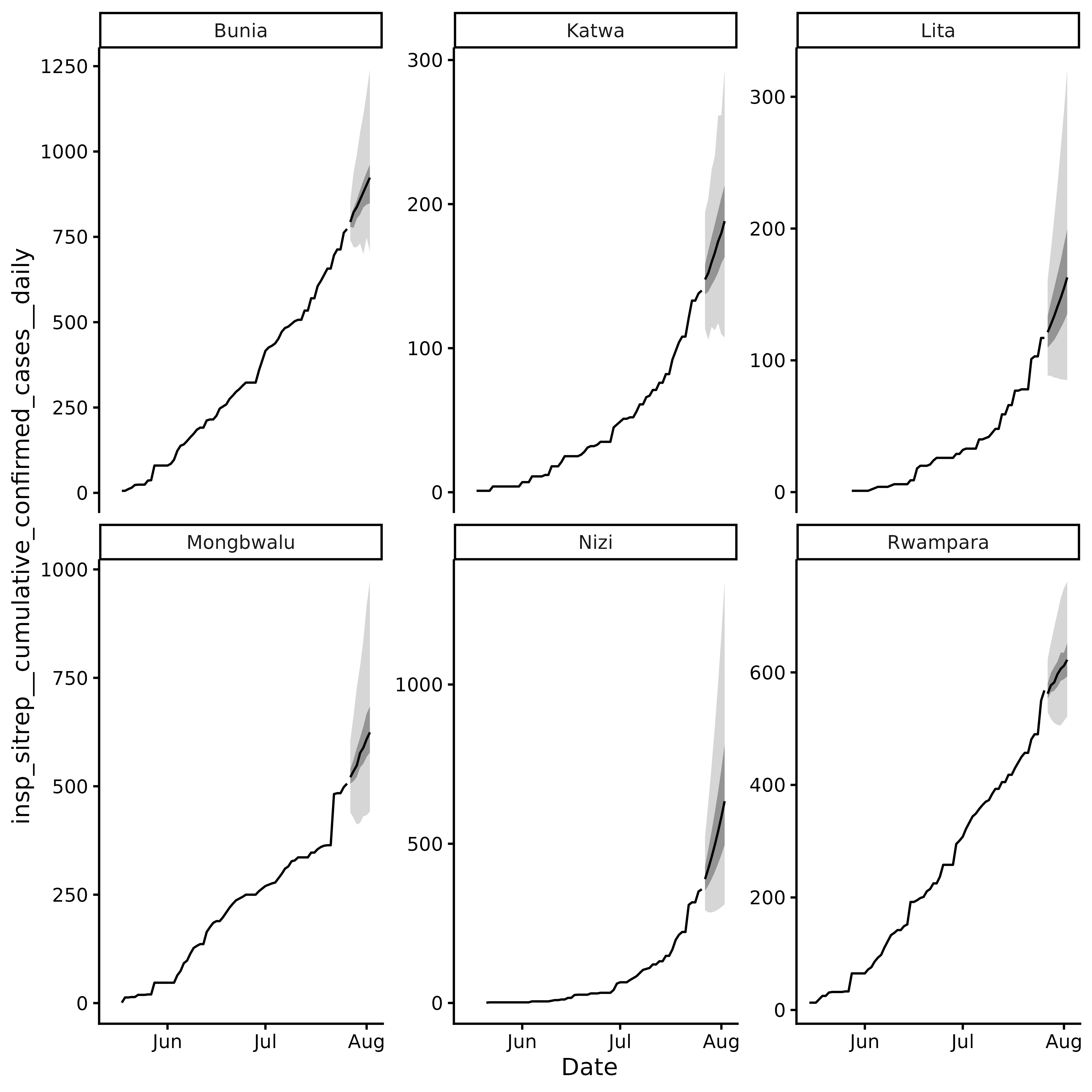
Ensemble forecast by location.
Use as_tibble() to build a custom plot:
fcast |>
  as_tibble() |>
  ggplot() +
  geom_ribbon(
    aes(x = target_end_date, ymin = lower, ymax = upper, fill = model_id),
    alpha = 0.2,
    show.legend = FALSE
  ) +
  geom_line(
    aes(x = target_end_date, y = median, colour = model_id),
    show.legend = TRUE
  ) +
  facet_wrap(~location, scales = "free") +
  geom_line(
    data = fcast$hub$oracle_output |>
      filter(target_end_date >= as.Date("2026-07-01")),
    aes(x = target_end_date, y = oracle_value),
    colour = "black"
  ) +
  theme_classic() +
  theme(
    legend.position = "bottom",
    legend.title = element_blank()
  )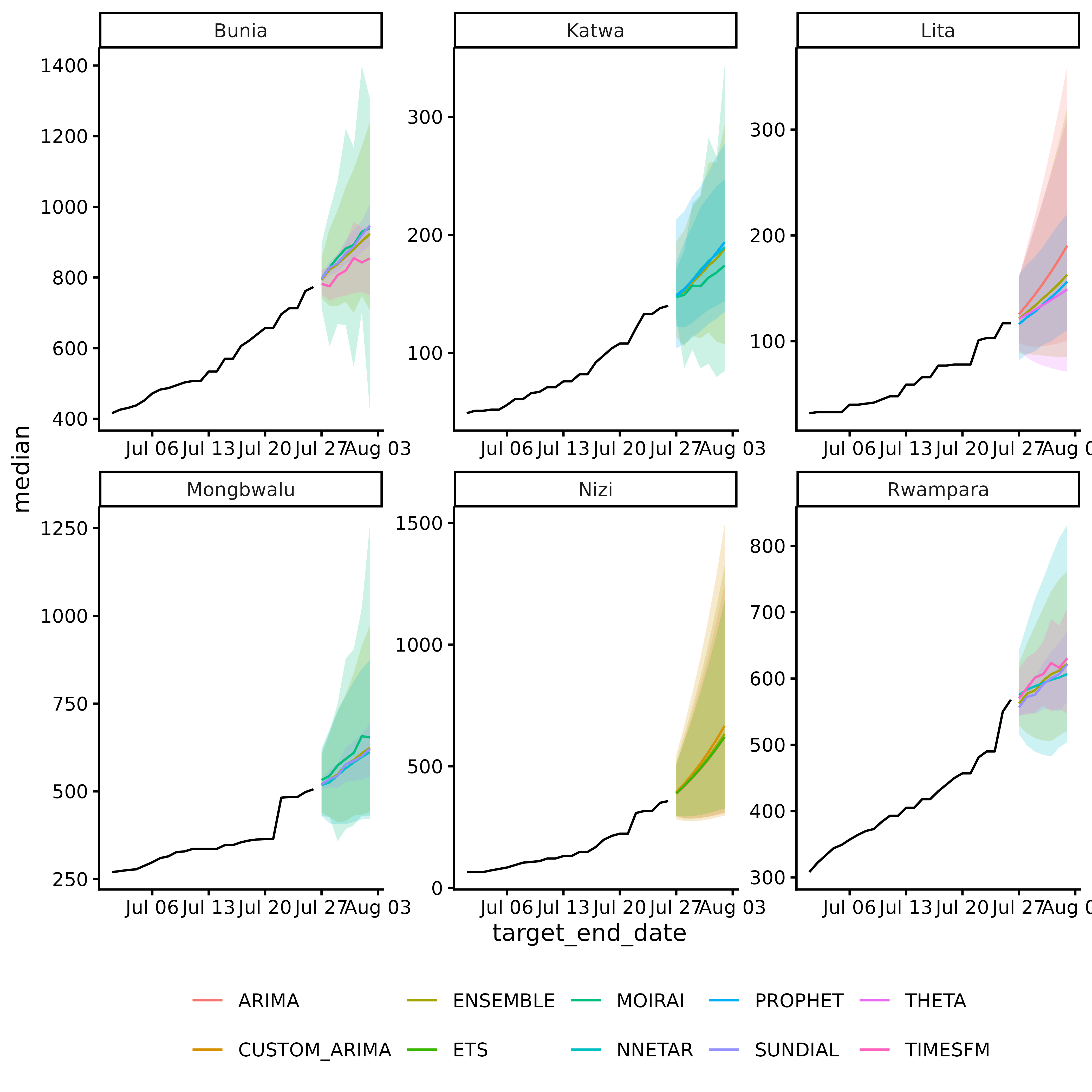
Forecasts by model with observed values in black.