9. Generate operational forecasts
Forecast the current influenza season using a trained model and the latest reported hospitalizations. Each forecasting cycle starts by updating surveillance data, then uses run_operational_flusight.py to inspect the observations, condition the model, and export FluSight CSVs, forecast PDFs, and sampled trajectories.
Reuse the selected checkpoint and its training dataset from the earlier steps. The observations and forecast date change each week; you can run this workflow without retraining. The figures below illustrate a reference date of November 29, 2025; set the date for your own forecast before sampling.
1. Update the surveillance data first
Before opening or running the forecasting notebook for a new forecast, update the local data checkouts from the research repository root:
The script pulls the local FluSight, NC collaboration, and Metrocast repositories listed in environment setup. Run it each time you prepare a new operational forecast, before the notebook constructs its ground-truth object.
GroundTruth.for_flusight reads local hospitalization data; it does not download the latest observations. For the 2025–2026 example, the current reader uses Flusight/2024-2025/FluSight-forecast-hub-official/target-data/target-hospital-admissions.csv. The directory name does not limit the seasons in that file. The notebook uses nogit=True, so setting data_date alone neither refreshes the data nor selects a historical Git revision.
2. Open the notebook
Complete environment setup and make the selected checkpoint and its training dataset available. Run from the research repository root. Open run_operational_flusight.py as a Jupytext notebook in your editor, or create an unexecuted notebook copy:
jupytext --to notebook run_operational_flusight.py --output run_operational_flusight.ipynb
jupyter lab run_operational_flusight.ipynb
Select Python (diffusion_torch) as the kernel. Run the cells interactively, setting the configuration before loading the model or starting sampling.
3. Choose the model and forecast date
The notebook uses scenario 868, 512 samples, and CoPaint configuration celebahq_noTTJ5. Set forecast_date to the intended forecast reference date; the checked-in notebook contains a fixed example date that must be changed for a new run.
To use the i868 candidate trained in the example experiment from step 3, set the configuration cell to:
scenario_id = 868
forecast_date = "2025-11-29"  # Replace with your forecast reference date.
config_name = "celebahq_noTTJ5"
batch_size = 512
experiment_name = "my-flu-experiment_training"
run_id = None
model_path = None
The notebook finds a finished run for that scenario in the named MLflow experiment. Use your selected scenario and experiment name. To select a particular training execution, set experiment_name = None and run_id to its MLflow run ID. To load a checkpoint file directly, set both experiment_name and run_id to None and set model_path to the .pth file.
The model/dataset cell also loads the scenario's training data to construct its transformations. Check that dataset_library() still points to the dataset used to train your checkpoint, and inspect the printed scenario string before sampling.
Three dates have different roles in this notebook:
| Setting | What it controls |
|---|---|
forecast_date |
The reference date chosen before sampling; it sets the observation-mask cutoff |
data_date |
The requested observation-data date; with nogit=True, the reader uses the current local files, so this value does not download or retrieve a historical snapshot |
submission_date |
The reference date written into filenames and exported forecast rows; the export cell calculates it separately from today's date |
The season is inferred from the date: for example, November 29, 2025 belongs to 2025–2026. For a forecast with observations through November 22, the November 29 row and following weeks are hidden. The plot in the next section shows that example.
4. Inspect the observations and mask
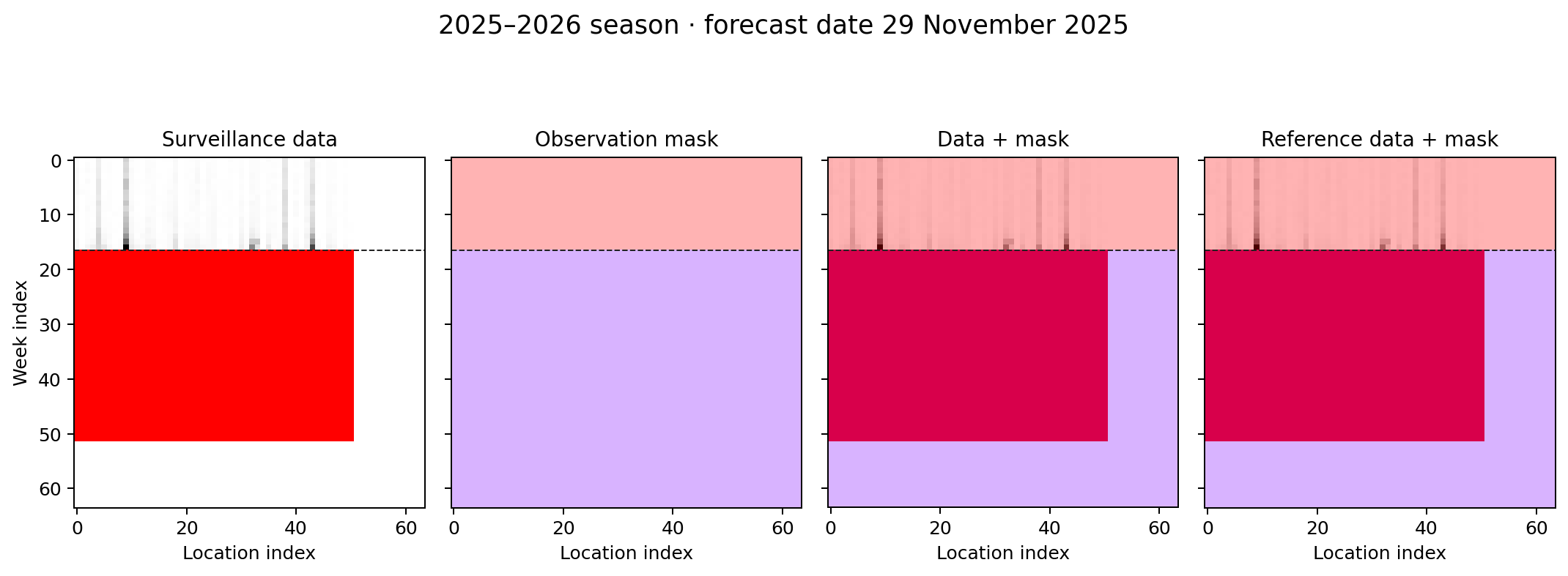
Early-season observation mask. This recreates the notebook's first graph, gt1.plot_mask(), using a surveillance snapshot from November 26, 2025, with observations through November 22. Rows are weeks and columns are locations on the padded 64 × 64 image grid. The mask is 1 for observed history and 0 for future weeks; its upper band is pink and its lower band is purple. The dashed line marks the forecasting boundary. Red entries in the data panels are missing values, while the extra rows and columns are padding. The last two panels overlay the same mask on the data and reference data; both use the same archived snapshot here, as in the notebook's nogit=True workflow.
Unlike the reconstruction experiments, the operational mask leaves the observed history available and hides the future. Inspect this graph before sampling to confirm the season, available observations, and forecast boundary.
Run the ground-truth cells after configuring the date. Confirm that the mask ends at the intended observation boundary and that the data panels contain the latest reported weeks. With nogit=True, this is the local surveillance snapshot you refreshed before opening the notebook.
5. Run inpainting
Run the sampler cells. They transform the observations, pass the data and mask to O_DDIMSampler, generate 512 trajectories, and transform the results back to hospitalization counts. The notebook then plots national and state forecasts. Review their agreement with recent observations and the spread of possible future trajectories before exporting.
6. Review the forecast plots
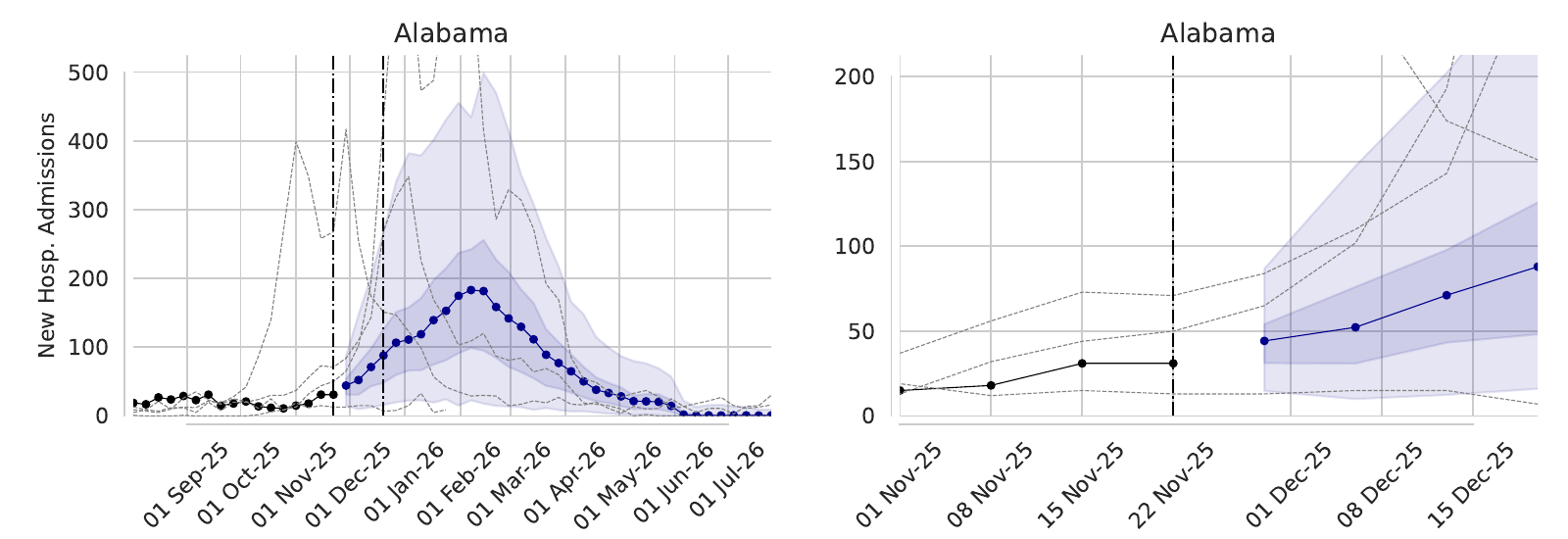
Saved operational forecast for Alabama, November 29, 2025. This is an excerpt from the original plot50-95.pdf in Flusight, showing the full season at left and the forecast window at right. Blue curves show medians and shaded bands show the 50% and 95% prediction intervals. Black points show available observations, gray dashed curves show earlier seasons, and vertical lines mark the forecast boundary and horizon in the full-season view.
Open the full original forecast PDF, including national and state panels
7. Export the forecast
The export cells choose the next Saturday from the current date as submission_date, refresh the ground-truth object from the local data, and write to operational_output/<submission_date>/. For a live run, keep the sampling date, observations, and submission reference date consistent. To replay a historical example, use its archived surveillance snapshot and explicitly set the export date and ground-truth cutoff to match; the default export cells use today's date even if forecast_date is historical.
For a run using an explicitly chosen reference date, replace the export cell's next-Saturday calculation with:
In the export cell that rebuilds GroundTruth.for_flusight, also set mask_date=pd.to_datetime(forecast_date) to keep the sampling cutoff. Use the same local surveillance snapshot for sampling and exporting. Rebuilding the ground-truth object does not rerun CoPaint: if you update the data or change the forecast cutoff, rerun the observation and sampling cells before exporting.
With the notebook's default prefix UNC_IDD-InfluPaint, the outputs are:
| Output | Contents |
|---|---|
<date>-UNC_IDD-InfluPaint.csv |
Location and national quantiles for the FluSight targets |
UNC_IDD-InfluPaint-<date>-plot50-95.pdf |
Median forecasts with 50% and 95% intervals |
UNC_IDD-InfluPaint-<date>-plotall.pdf |
Median forecasts with the full set of quantile bands |
<date>_fluforecasts_raw.npy |
Samples on the transformed model scale |
<date>_fluforecasts_transformed_inv.npy |
Sampled trajectories on the hospitalization scale |
<date>_forecasts_national.npy |
National trajectories aggregated from the samples |
The array files are written when save_raw_arrays=True. Open the CSV and check its reference_date, target_end_date, state codes, and quantile probabilities against the intended run. Horizons 0–3 should target the reference date and the next three weekly dates. Open both report PDFs to inspect the national and state forecasts. If the dates or observations are wrong, correct the notebook settings and regenerate the forecast and exports. Running the notebook creates local files; submission to FluSight is a separate action.
Paper reproducibility
If you have not completed training, you can start this stage with i868::m_U500cRx1224::ds_30S70M::tr_Sqrt::ri_No::3000.pth and datasets/training/TS_30S70M_2025-07-17.nc from the Zenodo reproducibility archive (archive README). Copy the NetCDF into training_datasets/, set scenario_id = 868, experiment_name = None, run_id = None, and model_path = "influpaint-paper/influpaint_paper_reproduction_data/i868::m_U500cRx1224::ds_30S70M::tr_Sqrt::ri_No::3000.pth". You still need to update surveillance data for the new forecast date.
Inspect a saved operational forecast
The example report and its preview are included on this page, so no model run is needed to inspect them. The original November 29 files are under Flusight/2025-2026/Flusight 2025-2026/2025-11-29/ in the local research archive. These are separate from the paper reproduction archive's earlier operational submissions in forecasts/operational/.
Sources for the example figures
The mask uses target-data/target-hospital-admissions.csv from revision aa25b8d92c06241d7e50dfb15b80fbc04f6483d5 in the local Flusight/2024-2025/my-hub-fork-for-submissions checkout. It is reconstructed from that archived surveillance snapshot, not extracted from a saved notebook output. The PDF is copied unchanged from Flusight/2025-2026/Flusight 2025-2026/2025-11-29/UNC_IDD-InfluPaint_celebahq_noTTJ5-2025-11-29-plot50-95.pdf; the inline preview crops its Alabama row.
Regenerate these documentation assets from the local source files with:
This calls the notebook's mask plotting method and uses Poppler's pdftoppm for the PDF preview. It does not generate new forecasts.