2. Create training data

Turn the source table from step 1 into complete training seasons with different mixtures of surveillance and simulated data. This lets you ask whether learning mainly from observed epidemics, mainly from simulations, or from a blend of both gives better forecasts.

Use dataset_creation/2-build_training_flu_datasets_ipynb.py to read Flusight/flu-datasets/all_datasets.parquet, choose the source proportions, fill out the week/location grid, and save four NetCDF datasets. Each training example becomes an image: weeks run down the rows, locations run across the columns, and pixel values describe epidemic intensity.

Open the Jupytext script as notebook cells and use the repository root as the working directory. Read Flusight/flu-datasets/all_datasets.parquet first. Run the cells in order: inspect source scales, set the mixing recipes, build frames, then save and plot the resulting datasets. The notebook writes training_datasets/TS_<mixture>_<today>.nc; note those filenames because you will select them in the training configuration in step 3.

Paper reproducibility

You can bypass this stage by getting its final outputs, the four July 17, 2025 NetCDF training datasets, directly from the Zenodo reproducibility archive (archive README).

If you have not completed step 1, you can start this stage with datasets/sources/all_datasets.parquet from the same archive. Copy it to Flusight/flu-datasets/all_datasets.parquet, then run the notebook below. This November source snapshot is not established as the original input to the July datasets; use the archived NetCDFs for the exact paper training inputs.

Use the exact paper inputs in influpaint-paper/influpaint_paper_reproduction_data/datasets/training/:

Bash

mkdir -p training_datasets
cp influpaint-paper/influpaint_paper_reproduction_data/datasets/training/TS_*_2025-07-17.nc training_datasets/

The files are TS_100S_2025-07-17.nc, TS_70S30M_2025-07-17.nc, TS_30S70M_2025-07-17.nc, and TS_100M_2025-07-17.nc. The batch configuration selects these dates explicitly.

1. Start from the source inventory

The input is the common table introduced in step 1: each row is a weekly value for a source, season, trajectory, and location. The broad source family is its first hierarchy level (datasetH1); a particular dataset or round/model/scenario combination is its second level (datasetH2). Grouping by those two labels, the season, and the trajectory ID collects all available weeks and locations for one source season.

Run the inventory cell immediately after the notebook loads the Parquet file. It prints how many sub-sources, seasons, and trajectories each family contains. In the saved example there are 13 FluView seasons, 7 FluSurv seasons, 160 flepiMoP season/trajectory groups, and 1,080 Flu Scenario Modeling Hub groups. The source inventory table explains those counts and the 57 sub-source labels.

This imbalance is why mixing is needed: using every source group once would give 20 surveillance groups alongside 1,240 simulated groups. To study how the balance affects forecasts, the notebook creates four training collections with different contributions from the observed and simulated sources. It does this by repeating source groups, completing their grids, and, where requested, rescaling their magnitudes.

2. Compare source scales

For each source season/trajectory, the notebook adds the values across available locations week by week, then records the largest weekly total. Comparing these peaks reveals the different scales of the sources: FluView measures influenza-like illness, while the other included families describe hospitalizations. Geographic coverage also differs, so these totals are not necessarily comparable national burdens.

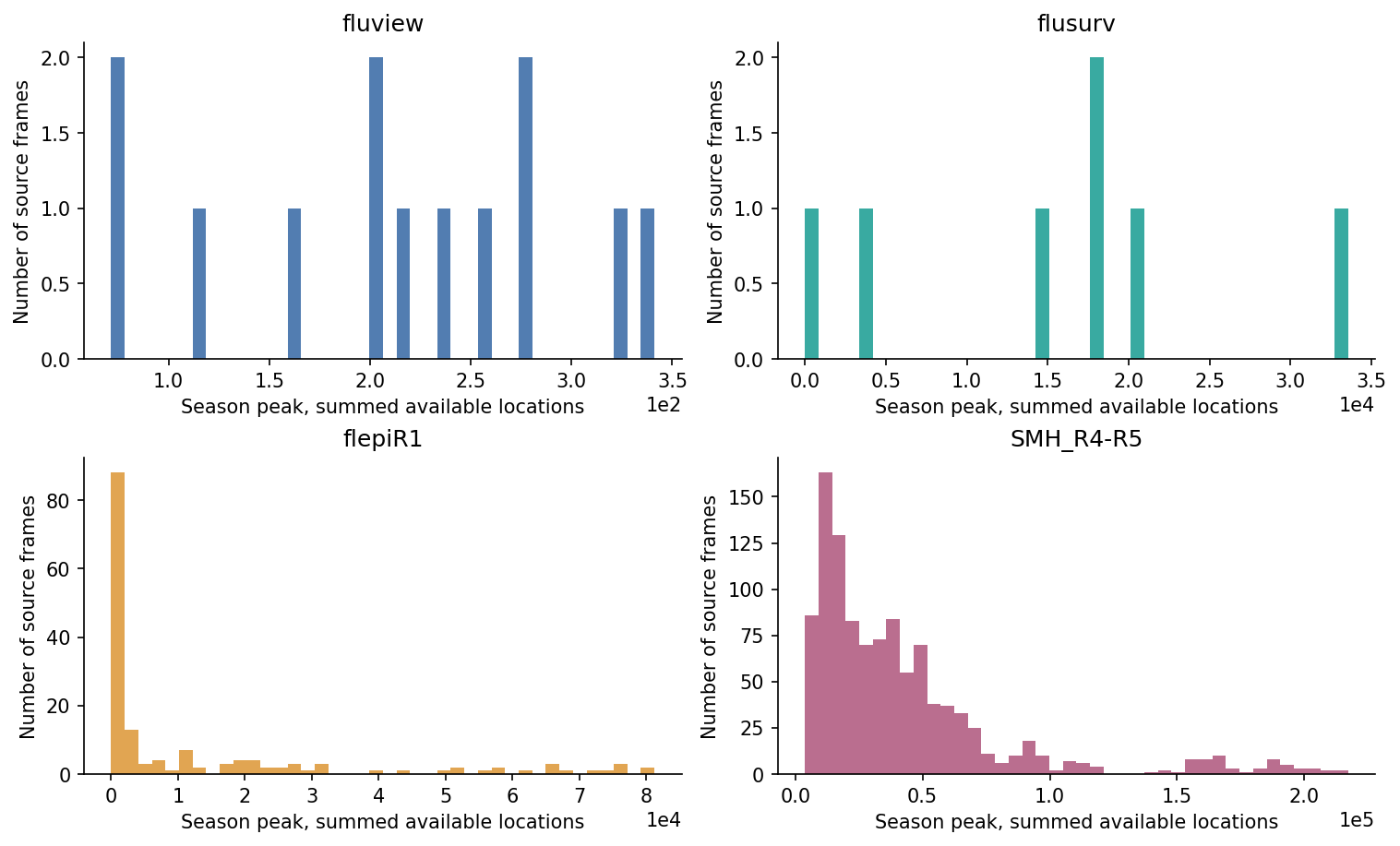
The notebook's peak calculation rendered from the archived Parquet table. Each histogram uses its own scale. Summed available locations do not necessarily provide equal geographic coverage across sources.

To bring FluView curves onto a hospitalization-like magnitude scale, the notebook draws target peaks from the Flu Scenario Modeling Hub simulations and rescales each FluView frame while retaining its epidemic shape. This is the to_scale=True option in the recipe. It is a training-data construction step, rather than a claim that influenza-like illness measurements are observed hospitalization counts.

3. Choose how much each source contributes

The four datasets range from surveillance only to simulations only. In their short filenames, S stands for surveillance and M for modeling: for example, 30S70M means a target mixture of 30% surveillance-derived training frames and 70% simulation-derived training frames. Those percentages describe the contribution of source frames to the training collection, not the fraction of hospitalizations, states, weeks, or pixels in a frame.

The two surveillance families are FluView and FluSurv. The two simulation families are flepiMoP round 1 and the Flu Scenario Modeling Hub rounds 4–5. Here is the full meaning of each supplied recipe:

Training collection	Short filename label	How its sources are weighted	Frames in the saved training file
Surveillance only	100S	Repeat each of the 13 FluView and 7 FluSurv source seasons 26 times	520
70% surveillance / 30% simulations	70S30M	Target 37% FluView + 33% FluSurv + 5% flepiMoP + 25% Scenario Modeling Hub	3,332
30% surveillance / 70% simulations	30S70M	Target 15% FluView + 15% FluSurv + 5% flepiMoP + 65% Scenario Modeling Hub	3,223
Simulations only	100M	Use each of the 160 flepiMoP and 1,080 Scenario Modeling Hub source groups once	1,240

The notebook records these recipes in the DATASET_GRIDS dictionary. It supports two ways to specify a collection:

• Repetition count (multiplier): how many times to use each source group. The surveillance-only recipe uses 26 repetitions, giving (13 + 7) × 26 = 520 frames. Repetition increases a source's training weight; it does not create additional observed seasons.
• Target share (proportion) and requested size (total): the desired fraction of frames from each family and the desired overall number of frames. Both mixed recipes request 3,000 frames. The mixer converts the target shares into source-repetition counts, so the final counts need not equal the requested size exactly.

For a concrete example, consider the request for 3,000 frames with 30% surveillance and 70% simulations. For each family, the mixer divides its requested count by the number of available source groups, rounds to an integer repetition count, and uses at least one repetition:

Source	Target share	Requested frames	Available source groups	Repetitions per group	Resulting frames
FluView	15%	450	13	35	455
FluSurv	15%	450	7	64	448
flepiMoP round 1	5%	150	160	1	160
Flu Scenario Modeling Hub	65%	1,950	1,080	2	2,160
Total	100%	3,000	1,260		3,223

These resulting counts match the main-source labels in the saved 30% surveillance / 70% simulations training file. They show why the mixture name expresses a target balance: whole-source repetition does not produce exactly the requested percentages. The percentages control how many frames each family contributes; individual values are rescaled separately by the peak-scaling step.

To change the balance, edit the four source shares in DATASET_GRIDS before the building loop. Keep the shares summing to one and use the same requested total for each family in a proportional recipe. To keep a source-only collection, use explicit repetition counts as in the first and last rows of the table.

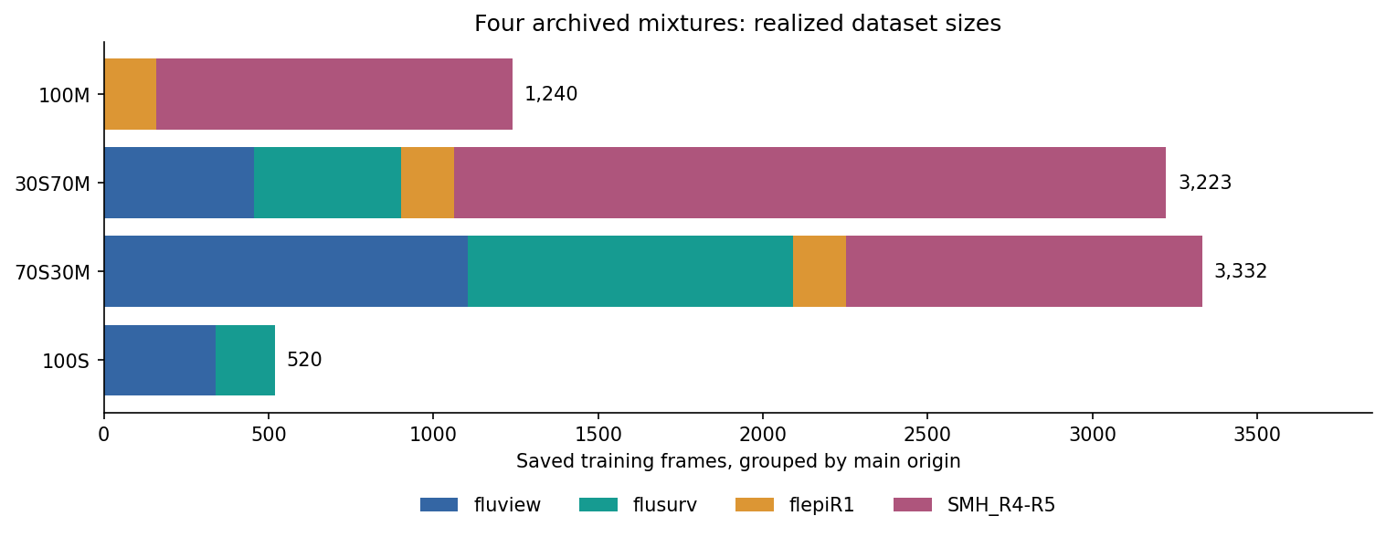
Counts read from the exact July 17 NetCDF files, grouped by each frame's main_origins attribute. Main origin summarizes frame provenance; filled locations can have different origins. The percentages are mixing targets, not guarantees of exact realized proportions. A requested size of 3,000 differs from the realized sample count and from 3,000 training epochs.

4. Complete each season's week/location grid

A frame is the collection of epidemic curves for one training example, laid out over all 53 season weeks and the 50 states plus DC. Source groups start with varying coverage; the frame builder fills the week/location grid before converting it to an image.

The notebook uses fill_missing_locations="random": when a location is absent from a source season, the mixer fills it with other season data. It records the contributing source in origin. The full frame can therefore contain curves from more than one source season, even though one origin is used to summarize it. The FluView rescaling described above also happens during frame construction.

influpaint/datasets/mixer.py performs this construction. The notebook then checks that every frame has weeks 1–53 and all required locations, and influpaint/utils/converters.py arranges it into the common array order. At this point the source table has become a collection of complete training examples.

5. See the season as an image

Each NetCDF file stores a stack of images with dimensions (sample, feature, season_week, place) and shape (N, 1, 64, 64). Here N is the number of training frames, sample indexes those frames, feature is the single incidence channel, season_week indexes rows, and place indexes location columns. This output sample index identifies a completed training image, rather than the original simulation trajectory ID in the source table. The first 53 rows and 51 columns contain the season; the remaining rows and columns are padding to make a 64 × 64 image. The same fixed location order is used in every image and saved in its coordinates; it is not an alphabetical ordering of state names.

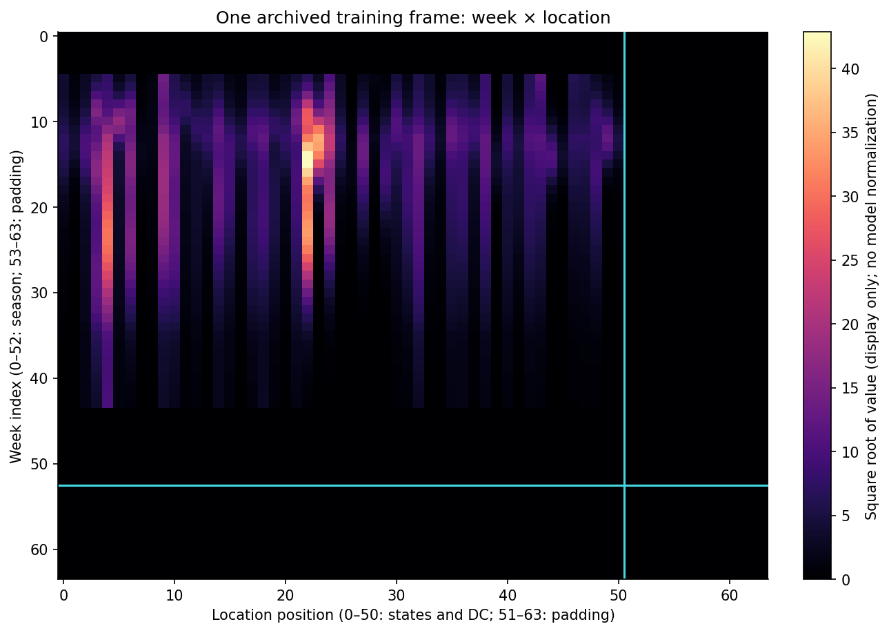
Sample 3000 from the archived 30S70M dataset. Cyan lines delimit padding. A square root makes the display readable; the model's full normalization is applied later by the training loader.

6. Return to epidemic curves for a sanity check

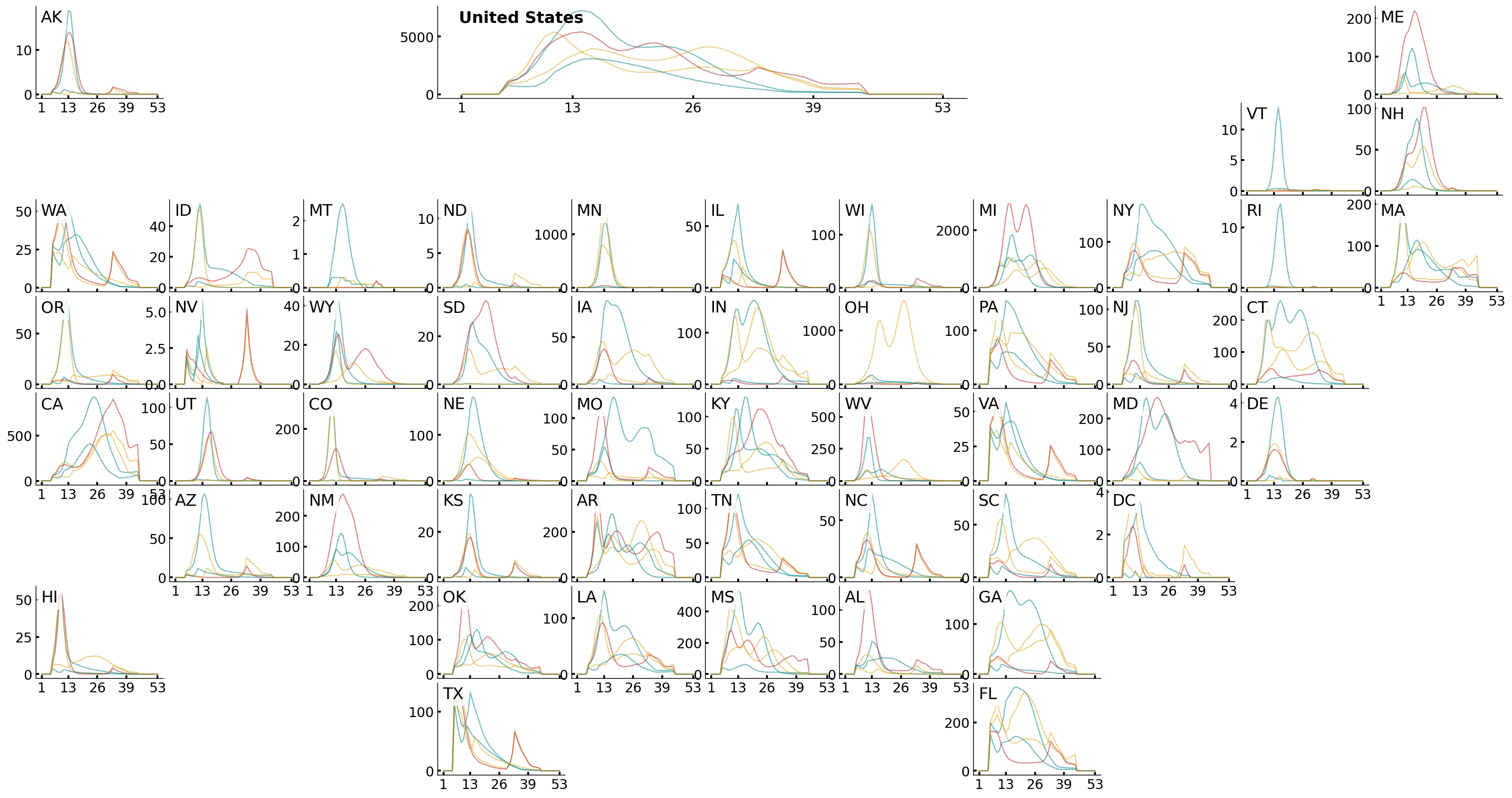
The notebook's final plot_us_grid call, using samples 3000–3004 from the saved 30S70M file. The geographic arrangement makes state trajectories readable; the model itself sees the fixed location-column order above.

Inspect both representations before training: the image should have the expected populated region and padding, and the state curves should have sensible shapes and magnitudes after scaling and gap filling. Compare the realized mixture sizes and source counts with your intended recipes.

Each saved NetCDF stores coordinates, main_origins, and mix_cfg alongside the values. Carry these files into step 3 and update dataset_library() to point to them. Training derives its transformations from the chosen dataset, and forecasting uses that same dataset to reconstruct the transformations.

Previous: 1. Gather source datasets · Next: 3. Train candidate models