1. Gather source datasets

The starting point for influpaint is a common table of weekly influenza measurements and simulated hospitalizations, saved as Flusight/flu-datasets/all_datasets.parquet. Each row holds one value for one location and week within a particular source, season, and trajectory. Grouping those rows gives epidemic curves; arranging the curves for all locations side by side will give the training images in step 2.

Assemble this table from four source families. Two describe observed epidemics through surveillance; two supply simulated epidemics from transmission models. The table gives them common column names and season labels while retaining their source identities and measurement scales. The first notebook, dataset_creation/1-gather_all_flu_datasets_ipynb.py, reads, inspects, and combines them.

Paper reproducibility

You can bypass source gathering by getting the saved output, datasets/sources/all_datasets.parquet, directly from the Zenodo reproducibility archive (archive README). Copy it into the location used by the walkthrough:

Bash

mkdir -p Flusight/flu-datasets
cp influpaint-paper/influpaint_paper_reproduction_data/datasets/sources/all_datasets.parquet Flusight/flu-datasets/all_datasets.parquet

The explanations and counts below describe this saved table. It is the November 7, 2025 source snapshot; the archive does not establish it as the original input to the July training files. For the paper's exact training images, use the saved NetCDF files described near the top of step 2. The Zenodo archive README records the reproduction inputs and provenance.

1. Understand the common table

The table is stored in Parquet, a format for saving tabular data. It has 2,535,111 rows and nine columns in the saved example. A row is a single weekly measurement, not a whole epidemic or a training image.

Column	What it means	Concrete example
datasetH1	First level of the source hierarchy: the broad source family	fluview identifies FluView surveillance; SMH_R4-R5 identifies the Flu Scenario Modeling Hub collection
datasetH2	Second level of the source hierarchy: a particular sub-source within that family	csp_flusurv identifies the processed FluSurv series; round4_USC-SIkJalpha_A-2023-08-14 identifies a Hub round, model, and scenario
fluseason	The starting year of the August-to-July season	2010 means the 2010–2011 season
sample	The trajectory identifier within a sub-source and season	Surveillance uses 1; a simulation source has multiple sample IDs for different modeled trajectories
location_code	The location to which the value belongs, usually a two-digit state/DC FIPS code	02 is Alaska; 37 is North Carolina
season_week	The week's position on the shared August-start season calendar, numbered 1–53	10 is the tenth week of the season, not the tenth week of the calendar year
week_enddate	The calendar date labeling the source's weekly value	2010-10-09
value	The measured or simulated quantity, still on its source's scale	FluView supplies an influenza-like illness measure; the other included sources supply observed-derived or modeled hospitalization values
fluseason_fraction	The date's fractional position through the August-to-July season	About 0.189 for the example date above

H1 and H2 describe where a record came from. H1 groups related data into a family; H2 distinguishes datasets within that family. A family with only one sub-source still has both columns. For FluView they both contain fluview; for FluSurv the family is flusurv and the selected processed sub-source is csp_flusurv.

A Hub sub-source needs a more detailed name. In round4_USC-SIkJalpha_A-2023-08-14, round4 identifies the modeling round, USC-SIkJalpha the submitted model, and A-2023-08-14 the scenario identifier. That H2 contains 20 sampled trajectories. Other scenarios from the same model get different H2 labels. These are the source models that generated training material; influpaint's candidate models are trained later in step 3.

From rows to a season

These are three actual rows from the saved table, with the optional fractional-season column omitted:

Source family (H1)	Sub-source (H2)	Season	Sample	Location	Season week	Week date	Value
fluview	fluview	2010	1	02 (Alaska)	10	2010-10-09	0.875146
fluview	fluview	2010	1	02 (Alaska)	11	2010-10-16	1.128270
fluview	fluview	2010	1	02 (Alaska)	12	2010-10-23	0.586042

Following the weeks for this location produces Alaska's epidemic curve. Keeping the same H1, H2, season, and sample while including the other locations gives one source season/trajectory group. Those four identifiers together identify a group; sample = 1 by itself is not unique across the table.

A source group can have missing weeks or locations. Step 2 fills out the required grid and turns groups into complete training images. The source table can also retain extra locations: the saved Hub collection includes national and territory records, while the training grid uses only the 50 states and DC.

2. Know which sources are included, and how many

Surveillance means measurements derived from actual influenza seasons. FluView reports influenza-like illness, while the included FluSurv series contains state-level hospitalization estimates prepared from FluSurv-NET data. Simulated data means hospitalization trajectories produced by transmission models under different assumptions and stochastic realizations. A trajectory is a sequence of weekly values across locations, representing one possible epidemic evolution.

The following counts come from executing the source-inventory cell at the beginning of the second notebook, dataset_creation/2-build_training_flu_datasets_ipynb.py, on the saved common table. The local input and the archived table agree. Counts describe the source collection before repetition, rescaling, gap filling, or image padding.

Source family and table label (H1)	What it contributes	Sub-sources (H2)	Season labels present	Trajectories per sub-source and season	Source season/trajectory groups
FluView surveillance — fluview	Historical influenza-like illness measurements	1: fluview	2010–2022 (13 seasons)	1 observed trajectory	13
FluSurv surveillance — flusurv	Hospitalization estimates prepared by the COVID Scenario Pipeline from FluSurv-NET	1: csp_flusurv	2015–2021 (7 seasons)	1 observed trajectory	7
flepiMoP round 1 simulations — flepiR1	Simulated influenza A and B hospitalizations, added together	1: flepiR1	2021 and 2022	80 sample IDs in each season	160
Flu Scenario Modeling Hub rounds 4–5 — SMH_R4-R5	Hospitalization trajectories from multiple submitted models and scenarios	54	2023 or 2024, depending on sub-source	20; each H2 covers one season	1,080
Total	4 source families	57			1,260

Thus the collection contains 20 surveillance season groups and 1,240 simulated season/trajectory groups. The flepiMoP count is 80 sampled trajectories split across two season labels, giving 160 groups; it does not mean 160 independent simulations. These groups are not necessarily complete seasons yet.

The Hub's 54 H2 labels are round/model/scenario combinations, not 54 distinct models. Their breakdown is:

Round	Model names in the saved collection	H2 combinations	Season/trajectory groups
4	USC-SIkJalpha, NotreDame-FRED, MOBS_NEU-GLEAM_FLU	3 models × 6 scenarios = 18	18 × 20 samples = 360
5	USC-SIkJalpha, NotreDame-FRED, MOBS_NEU-GLEAM_FLU, SigSci-SWIFT, UVA-EscapeFlu, ACCIDDA-FlepiMoP	6 models × 6 scenarios = 36	36 × 20 samples = 720

The second notebook's inventory prints datasetH1, the number of H2 labels (nH2), and then each H2's row count, number of seasons, sample count, and frame count. For example:

Text Only

datasetH1: fluview, nH2= 1
 - datasetH2: fluview, shape: (30834, 9), years: 13, samples: 1 ===> n_frames=13
datasetH1: flepiR1, nH2= 1
 - datasetH2: flepiR1, shape: (191760, 9), years: 2, samples: 80 ===> n_frames=160

Here shape: (30834, 9) means 30,834 weekly records and nine columns. n_frames=13 counts season/trajectory groups, not weekly records. Run this inventory cell after loading your own table to see the corresponding counts before choosing mixture sizes in step 2.

3. Open the gathering notebook

To assemble the table from its sources, open dataset_creation/1-gather_all_flu_datasets_ipynb.py. It uses Jupytext's # %% cell format. Open it as a notebook in your editor, or create an unexecuted Jupyter copy:

Bash

jupytext --to notebook dataset_creation/1-gather_all_flu_datasets_ipynb.py --output dataset_creation/1-gather_all_flu_datasets.ipynb

Run cells from the repository root. The notebook defaults to download=False, reading cached upstream files. Prepare the upstream checkouts listed in environment setup, then follow the source-specific preparation cells. The source readers rename each source's time, location, and measurement fields into the common columns above and attach the source and trajectory identifiers.

4. Inspect the observed surveillance seasons

The notebook places dates on the August-start calendar and standardizes location labels. The season-overlap plots let you compare timing, magnitude, and coverage before mixing sources.

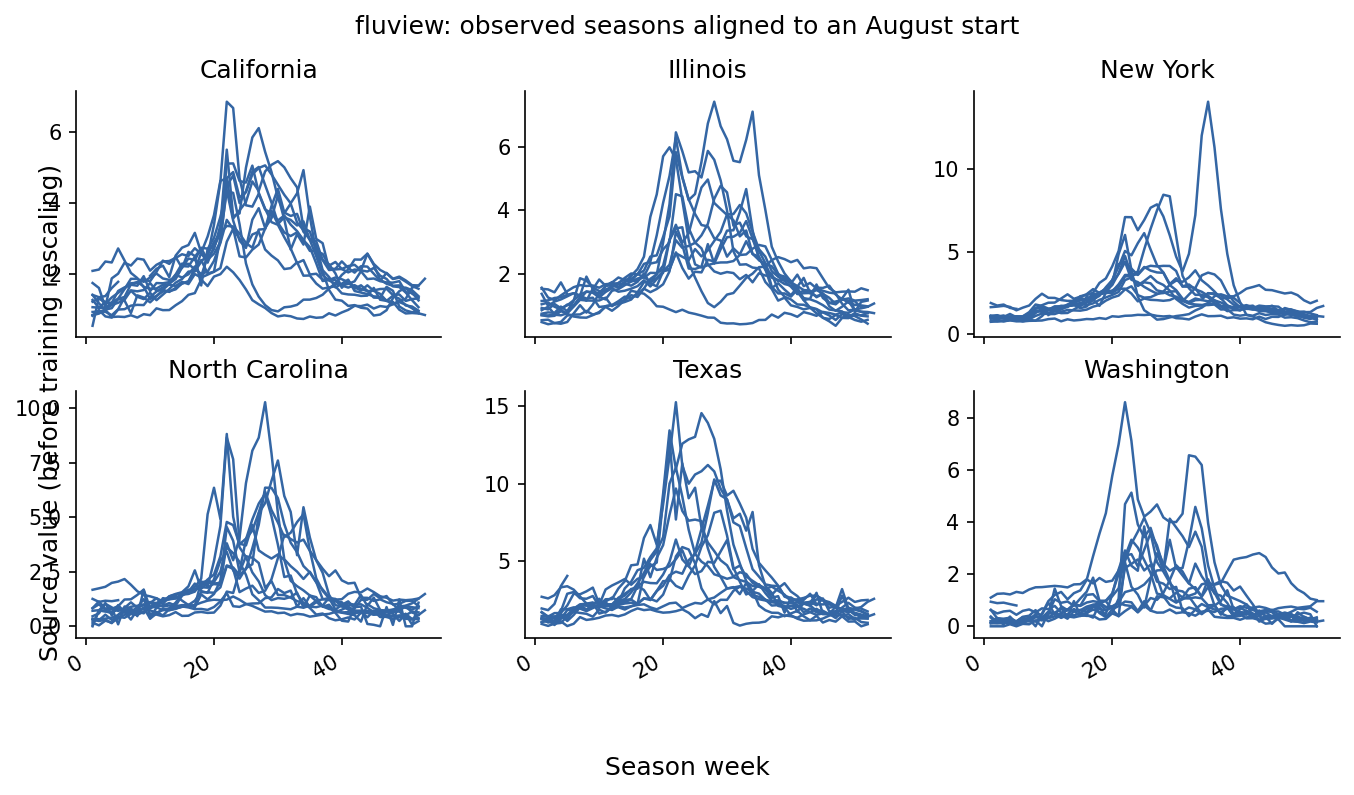
FluView influenza-like illness curves for six states, with one line per observed season. They retain the FluView measurement scale; the next step rescales their magnitudes before combining them with hospitalization trajectories.

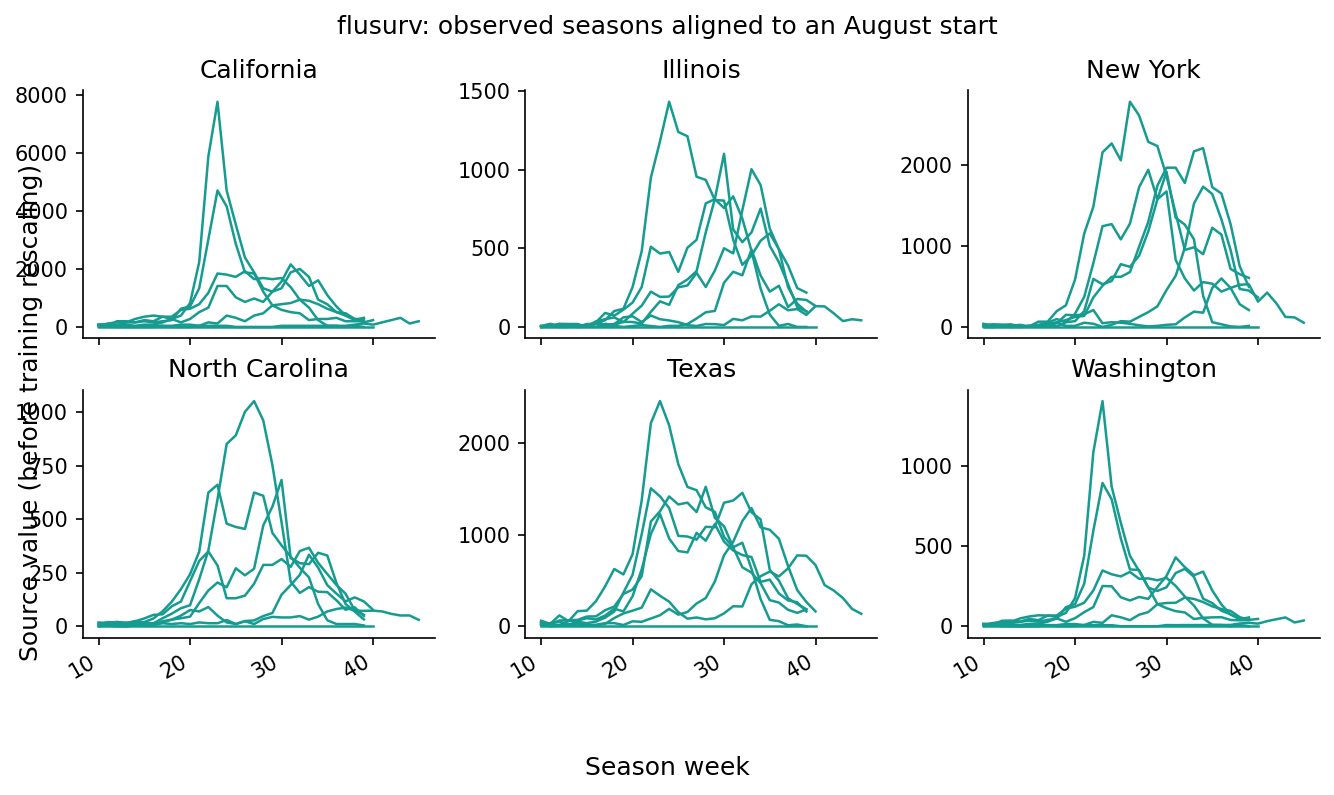
The processed FluSurv hospitalization series, labeled csp_flusurv in H2. The notebook also inspects Delphi FluSurv, but only the COVID Scenario Pipeline series enters the final common table.

5. Add simulated epidemics

The notebook reads Flu Scenario Modeling Hub rounds 4–5, excludes PSI-M2 because its sample numbering is inconsistent across locations, and keeps 20 trajectories per included round/model/scenario combination. It also reads the flepiMoP round 1 simulations, adds influenza A and B hospitalizations, and selects 80 sample IDs. These sample selections are random, so a fresh run can select different trajectories.

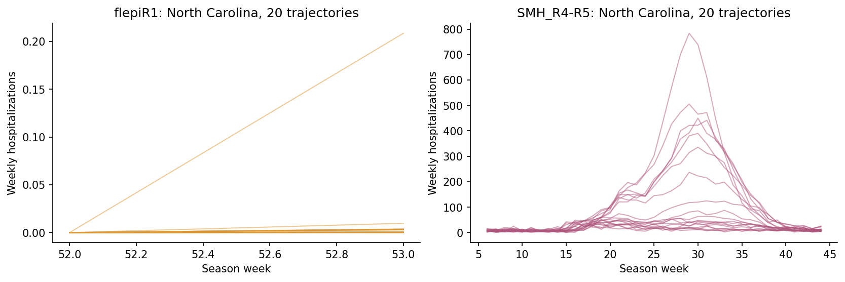
Twenty North Carolina trajectories from each simulation family in the saved table. These show the range of epidemic shapes and magnitudes the simulations add to the observed seasons.

6. Save the source collection and continue

The notebook concatenates the four families and writes Flusight/flu-datasets/all_datasets.parquet. At this point the rows have a common structure, but their measurement scales and spatial/temporal coverage still differ. Step 2 addresses those differences and chooses how often each source contributes to training.

The NHSN (National Healthcare Safety Network) cells separately prepare observed hospitalizations at influpaint/data/nhsn_flusight_past.csv. Those observations supply history and evaluation targets; they are outside the four training-source families in the common table.

Run the standard cells through the Parquet save. The notebook's intentional assert False marks the boundary before optional custom-data experiments. Then open the second notebook, run its source inventory, and continue to step 2 to build the training images.

Previous: Start here · Next: 2. Create training data