7. Reconstruct missing observations

Use the selected model to reconstruct missing states, missing weeks, and gaps within a season. Starting with the checkpoint and CoPaint setting selected in step 6, hide whole states, a stretch of weeks, or alternating blocks, then generate trajectories conditioned on the entries that remain visible.

The workflow is the same as forecasting: prepare data and a mask, sample with fixed model weights, and compare the generated values with the hidden observations. Only the observation pattern changes.

Paper reproducibility

You can bypass this stage by getting its final outputs directly from the Zenodo reproducibility archive (archive README): the reconstruction samples, masks, and ground-truth arrays under forecasts/masks/.

If you have not completed the previous stages, these saved arrays let you inspect the six paper reconstruction experiments directly. Running new reconstructions with the script below still requires a finished MLflow training run and its matching training dataset; the script is configured to load that run rather than the standalone archived checkpoint.

Use influpaint-paper/influpaint_paper_reproduction_data/forecasts/masks/. Each experiment directory contains fluforecasts_ti.npy, mask.npy, and ground_truth.npy. For example, influpaint-paper/influpaint_paper_reproduction_data/forecasts/masks/missing_nc_season2023/fluforecasts_ti.npy contains the North Carolina reconstruction ensemble.

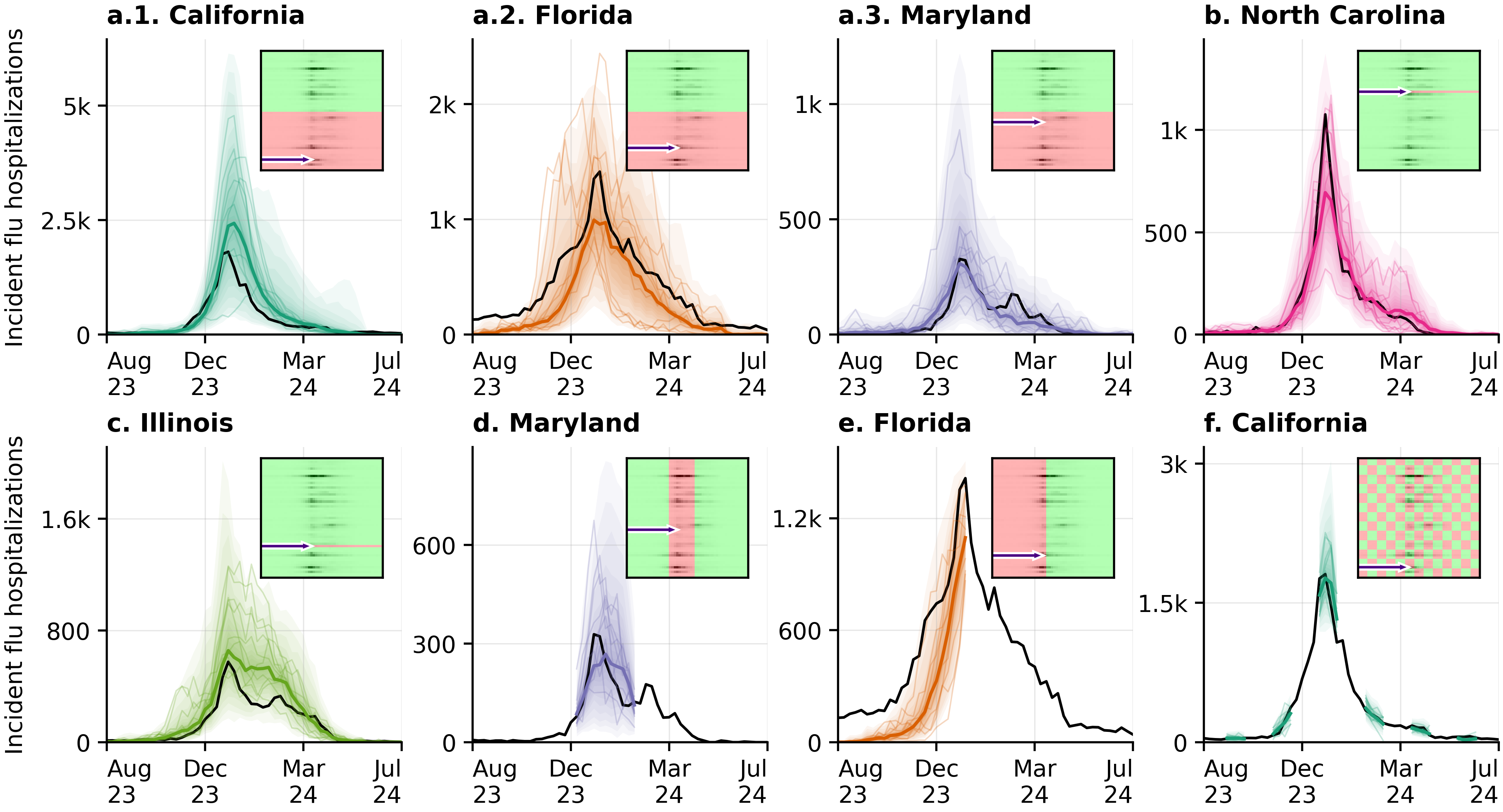
Figure 4 — Reconstruction with different observation masks. Each inset shows the entries supplied to the model in green and the hidden entries in red. Black curves show observed hospitalizations; colored lines and fans show reconstructed medians and predictive quantiles. The same trained model handles missing states, midseason gaps, missing early weeks, and checkerboard patterns by changing the mask at sampling time.

1. Define which observations to hide

A forecasting mask hides future weeks. These experiments instead hide whole locations, an internal time interval, past weeks, or scattered blocks. CoPaint conditions on the remaining entries and generates the missing portion using the same selected model.

A mask is an array with the same channel/week/location dimensions as a season image. Set an entry to 1 to supply its observed value to CoPaint, or 0 to withhold it. The full truth array remains available for comparison after sampling. Hiding North Carolina therefore means setting its entire column to 0, while keeping the other states available.

Set the following variables in main_training/mask_experiments.py:

Variable	Supplied value	What to change for your experiment
`EXPERIMENT_NAME`	`paper-2025-07-22_training`	The MLflow experiment containing your selected training run
`SCENARIO_ID`	`868`	The candidate's architecture, dataset, and preprocessing recipe
`CONFIG_NAME`	`celebahq_noTTJ5`	The CoPaint setting selected during forecast evaluation
`BATCH_SIZE`	`512`	Number of reconstruction trajectories per mask
`for season_first_year in [...]`	`["2023", "2024"]`	Season start years to reconstruct; `"2023"` means 2023–2024

The script loads the first matching finished training run returned for the chosen scenario. Check the printed RUN_ID before sampling, especially if the experiment contains more than one training execution for that scenario.

Define a mask in the season loop

The masks dictionary names the reconstructions to run. This example keeps all entries except North Carolina, whose FIPS code is 37:

Python

mask = np.ones((CHANNELS, IMAGE_SIZE, IMAGE_SIZE))
mask = mask_subpop(mask, ["37"], gt1.season_setup)
masks["missing_nc"] = mask

To hide weeks across all locations, use mask_dates. For example, inside the season loop:

Python

mask = np.ones((CHANNELS, IMAGE_SIZE, IMAGE_SIZE))
mask = mask_dates(
    mask,
    [(f"{season_first_year}-12-07", f"{int(season_first_year) + 1}-01-07")],
    gt1.season_setup,
)
masks["missing_midseason"] = mask

This hides the season-week rows containing December 7 through January 7, including both endpoint weeks. For a gap limited to selected states, use mask_dates_for_subpop with the date interval and state codes. _checkerboard_mask(4, 4) alternates hidden and observed blocks of four week rows by four location columns. Those columns follow the model's location order; they are not geographic squares on a map.

The script plots the masks before sampling. Inspect the image itself: dates are converted into season-week positions, so confirm that the intended weeks and state columns are hidden. The saved mask.npy records what was actually supplied to the sampler.

2. Run the reconstruction experiments

Adapt the Python environment and Slurm resources in the launcher, then submit from the repository root:

Bash

sbatch main_training/mask_experiments.run

The launcher runs python -m main_training.mask_experiments from the repository root. One job processes every mask in the masks dictionary for each selected season. It creates mask_experiments_<scenario>_<configuration>/, with subdirectories named <mask_name>_season<year>. It requests one GPU, 64 GB RAM, and ten hours on the original Longleaf configuration. The module retrieves i868 from paper-2025-07-22_training and uses celebahq_noTTJ5.

3. Compare reconstruction with withheld truth

Archived directory under `forecasts/masks/`	Hidden entries
`missing_half_subpop_season2023`	The first 25 of the 51 locations in the model's column order
`missing_nc_season2023`	North Carolina
`missing_il_season2023`	Illinois
`missing_midseason_biggap_season2023`	A midseason interval
`missing_past_season2023`	The early season
`missing_checkerboard_4x4_season2023`	Alternating four-week by four-location blocks

In mask.npy, 1 means observed and 0 means hidden. The mask and saved truth have shape (1,64,64); reconstruction arrays have shape (512,1,64,64). Figure 4 compares the generated trajectories against the saved, untransformed truth for the 2023–2024 season. Look at the hidden regions when assessing reconstruction: how much does the model recover from neighboring weeks or other locations, and how does uncertainty widen where evidence is sparse? For example, the North Carolina reconstruction tests whether the model can recover that state's epidemic using observations from the other states. A midseason gap also gives the model observations after the gap; it tests interpolation rather than a forecast made before those later observations existed.

Keep fluforecasts_ti.npy, mask.npy, and ground_truth.npy together. To reproduce Figure 4 from those saved files, follow the paper-figure instructions.

Previous: 6. Score forecasts · Next: 8. Reproduce paper figures