
Flexible Location Layers in imuGAP
Source:vignettes/user_specified_layers.Rmd
user_specified_layers.RmdOverview
The imuGAP package estimates the underlying vaccination
process model across nested population hierarchies (e.g. a state divided
into counties, counties into schools) and uses the fitted model to
predict coverage across resolution levels. A key strength of
imuGAP is support for flexible location
layers: the process model dynamically scales its hierarchical
depth to match the population structure you provide. If you supply only
aggregate state-wide data, the model estimates a 1-layer structure;
adding counties expands it to 2 layers; adding schools creates a 3-layer
hierarchy, and so forth.
Whatever the data resolution, imuGAP canonicalizes the
population tree, maps parent-child relationships across layers, and
estimates hierarchical location offset parameters for each resolution
level (beyond fully aggregated populations).
This vignette demonstrates:
- Exploring arbitrary location hierarchies and verifying layer depths.
- Constructing models for 1-layer (state-level only), 2-layer (state and county), and 3-layer (state, county, and school) datasets.
- Fitting and comparing parameter recovery and projected cohort trajectories across different layer resolutions.
The Example Location Hierarchy
Let’s first inspect the full hierarchy available in
locations_sim:
| Scruggs County | Simone County | Watson County |
|---|---|---|
| Chickadee Elementary | Egret Elementary | Meadowlark School |
| Nuthatch Academy | Cardinal Academy | Goldfinch Elementary |
| Blue Heron School | Bunting School | Mockingbird Academy |
| Flycatcher Elementary | Tanager Academy | Kinglet Learning Center |
| Bluebird Learning Center | Oriole Youth Academy | Vireo School |
| Catbird Academy | Grosbeak Learning Center | Kingfisher Academy |
| Finch Elementary | Junco Elementary | Cormorant Elementary |
| Sparrow School | ||
| Towhee Children’s Academy | ||
| Warbler Elementary |
Most of our examples focus on using the higher resolution dataset
(i.e. including 3 layers, or down to schools). For this demonstration,
let’s create some alternative location data corresponding
to different data availability. Here, we’re using the convenient layer
information created by canonicalize_locations, but in real
applications you would of course only have the locations you have. These
filtered views simulate having high to low resolution data, correspond
to all the locations in the table (locs_3layer), the state
and county locations (locs_2layer), or just the state
(locs_1layer).
locs_3layer <- canonicalize_locations(locations_sim) # all the data
locs_2layer <- locs_3layer[layer <= 2] # state and county only
locs_1layer <- locs_3layer[layer <= 1] # state only
Similarly, you can filter observations and associated metadata (i.e. populations) to match each location resolution:
data("observations_sim", package = "imuGAP")
data("populations_sim", package = "imuGAP")
data("latent_params_sim", package = "imuGAP")

# 3-Layer views (State, County, School)
# 1. Filter populations to locations present in locs_3layer
pops_3layer <- populations_sim[loc_id %in% locs_3layer$loc_id]
# 2. Extract relevant observations corresponding to filtered populations
obs_3layer <- observations_sim[obs_id %in% pops_3layer$obs_id]
# 3. Confirm extracted observations don't have unpresent locations in original population data
stopifnot(!populations_sim[obs_id %in% obs_3layer$obs_id, any(!loc_id %in% locs_3layer$loc_id)])

# 2-Layer views (State and County)
# 1. Filter populations to locations present in locs_2layer
pops_2layer <- populations_sim[loc_id %in% locs_2layer$loc_id]
# 2. Extract relevant observations corresponding to filtered populations
obs_2layer <- observations_sim[obs_id %in% pops_2layer$obs_id]
# 3. Confirm extracted observations don't have unpresent locations in original population data
stopifnot(!populations_sim[obs_id %in% obs_2layer$obs_id, any(!loc_id %in% locs_2layer$loc_id)])

# 1-Layer views (State only)
# 1. Aggregate and filter populations to State level (locs_1layer)
pops_1layer <- copy(populations_sim)[, loc_id := "State"]
pops_1layer <- pops_1layer[, .(weight = sum(weight)), by = .(obs_id, loc_id, cohort, age, dose)]
pops_1layer <- pops_1layer[loc_id %in% locs_1layer$loc_id]
# 2. Extract relevant observations corresponding to filtered populations
obs_1layer <- observations_sim[obs_id %in% pops_1layer$obs_id]
# 3. Confirm extracted observations don't have unpresent locations in population data
stopifnot(!pops_1layer[obs_id %in% obs_1layer$obs_id, any(!loc_id %in% locs_1layer$loc_id)])
2. Fitting the Model
To fit the model at different resolutions looks basically the same: just use 1-layer, 2-layer, or 3-layer location inputs. Note that no other setting tweaks are required, but these can take some time to run; if following along, you probably want to load the results from the package data.
st_opts <- stan_options(iter = 1000, chains = 4, seed = 1L)

# various layer fits
fit_3layer <- sampling(obs_3layer, pops_3layer, locs_3layer, stan_opts = st_opts)
fit_2layer <- sampling(obs_2layer, pops_2layer, locs_2layer, stan_opts = st_opts)
fit_1layer <- sampling(obs_1layer, pops_1layer, locs_1layer, stan_opts = st_opts)
To load precomputed results, get the following items from package data:
data("fit_sim", package = "imuGAP")
data("fit_sim_2layer", package = "imuGAP")
data("fit_sim_1layer", package = "imuGAP")

fit_sim_2layer
#> An imuGAP model fit (`imugap_fit`):
#>   Hierarchy:    4 locations across 2 layers (root: 'State')
#>   Observations: 841 total (775 uncensored, 66 right-censored)
#>
#> Inference for Stan model: bspline_static_zero_halley2_logit.
#> 4 chains, each with iter=125; warmup=0; thin=1;
#> post-warmup draws per chain=125, total post-warmup draws=500.
#>
#>                       mean se_mean   sd      2.5%       25%       50%       75%
#> beta_bs[1]           -1.67    0.00 0.03     -1.74     -1.69     -1.67     -1.64
#> beta_bs[2]           -1.88    0.00 0.05     -2.00     -1.92     -1.88     -1.84
#> beta_bs[3]           -2.47    0.00 0.09     -2.64     -2.53     -2.47     -2.41
#> beta_bs[4]           -3.23    0.00 0.11     -3.47     -3.30     -3.23     -3.15
#> beta_bs[5]           -2.61    0.00 0.09     -2.80     -2.67     -2.61     -2.55
#> sigma_layer[1]        0.66    0.02 0.33      0.24      0.41      0.58      0.85
#> lambda_raw[1]         1.01    0.00 0.03      0.96      0.99      1.01      1.03
#> lambda_raw[2]         1.01    0.00 0.01      0.98      1.00      1.01      1.02
#> raw_phi_root[1]      -1.67    0.00 0.03     -1.74     -1.69     -1.67     -1.64
#> raw_phi_root[2]      -1.71    0.00 0.03     -1.77     -1.73     -1.71     -1.70
#> raw_phi_root[3]      -1.76    0.00 0.02     -1.81     -1.78     -1.76     -1.74
#> raw_phi_root[4]      -1.81    0.00 0.02     -1.86     -1.83     -1.81     -1.79
#> raw_phi_root[5]      -1.86    0.00 0.02     -1.91     -1.88     -1.86     -1.84
#> raw_phi_root[6]      -1.92    0.00 0.03     -1.97     -1.93     -1.92     -1.90
#> raw_phi_root[7]      -1.97    0.00 0.03     -2.02     -1.99     -1.97     -1.95
#> raw_phi_root[8]      -2.03    0.00 0.03     -2.08     -2.05     -2.03     -2.01
#> raw_phi_root[9]      -2.09    0.00 0.03     -2.14     -2.11     -2.09     -2.07
#> raw_phi_root[10]     -2.15    0.00 0.03     -2.21     -2.17     -2.15     -2.13
#> raw_phi_root[11]     -2.21    0.00 0.03     -2.27     -2.23     -2.21     -2.19
#> raw_phi_root[12]     -2.28    0.00 0.03     -2.34     -2.30     -2.28     -2.25
#> raw_phi_root[13]     -2.34    0.00 0.03     -2.41     -2.36     -2.34     -2.32
#> raw_phi_root[14]     -2.41    0.00 0.04     -2.48     -2.43     -2.41     -2.38
#> raw_phi_root[15]     -2.48    0.00 0.04     -2.55     -2.50     -2.48     -2.45
#> raw_phi_root[16]     -2.55    0.00 0.04     -2.62     -2.57     -2.55     -2.52
#> raw_phi_root[17]     -2.62    0.00 0.04     -2.70     -2.64     -2.62     -2.59
#> raw_phi_root[18]     -2.68    0.00 0.04     -2.77     -2.71     -2.68     -2.65
#> raw_phi_root[19]     -2.75    0.00 0.05     -2.84     -2.78     -2.75     -2.71
#> raw_phi_root[20]     -2.81    0.00 0.05     -2.91     -2.84     -2.81     -2.77
#> raw_phi_root[21]     -2.86    0.00 0.06     -2.97     -2.89     -2.86     -2.82
#> raw_phi_root[22]     -2.90    0.00 0.06     -3.02     -2.93     -2.90     -2.86
#> raw_phi_root[23]     -2.92    0.00 0.06     -3.05     -2.96     -2.92     -2.88
#> raw_phi_root[24]     -2.94    0.00 0.06     -3.06     -2.98     -2.94     -2.90
#> raw_phi_root[25]     -2.94    0.00 0.06     -3.06     -2.98     -2.93     -2.90
#> raw_phi_root[26]     -2.92    0.00 0.06     -3.04     -2.95     -2.91     -2.88
#> raw_phi_root[27]     -2.88    0.00 0.06     -3.00     -2.91     -2.87     -2.84
#> raw_phi_root[28]     -2.81    0.00 0.06     -2.94     -2.85     -2.81     -2.77
#> raw_phi_root[29]     -2.73    0.00 0.07     -2.87     -2.77     -2.72     -2.68
#> raw_phi_root[30]     -2.61    0.00 0.09     -2.80     -2.67     -2.61     -2.55
#> mu_offset[1,1]       -0.04    0.00 0.00     -0.05     -0.04     -0.04     -0.04
#> mu_offset[2,1]       -0.04    0.00 0.00     -0.05     -0.04     -0.04     -0.04
#> mu_offset[3,1]       -0.04    0.00 0.00     -0.05     -0.05     -0.04     -0.04
#> mu_offset[4,1]       -0.04    0.00 0.00     -0.05     -0.05     -0.04     -0.04
#> mu_offset[5,1]       -0.04    0.00 0.00     -0.05     -0.05     -0.04     -0.04
#> mu_offset[6,1]       -0.05    0.00 0.00     -0.06     -0.05     -0.05     -0.04
#> mu_offset[7,1]       -0.05    0.00 0.00     -0.06     -0.05     -0.05     -0.04
#> mu_offset[8,1]       -0.05    0.00 0.00     -0.06     -0.05     -0.05     -0.04
#> mu_offset[9,1]       -0.05    0.00 0.01     -0.06     -0.05     -0.05     -0.04
#> mu_offset[10,1]      -0.05    0.00 0.01     -0.06     -0.05     -0.05     -0.04
#> mu_offset[11,1]      -0.05    0.00 0.01     -0.06     -0.05     -0.05     -0.05
#> mu_offset[12,1]      -0.05    0.00 0.01     -0.06     -0.05     -0.05     -0.05
#> mu_offset[13,1]      -0.05    0.00 0.01     -0.06     -0.05     -0.05     -0.05
#> mu_offset[14,1]      -0.05    0.00 0.01     -0.06     -0.05     -0.05     -0.05
#> mu_offset[15,1]      -0.05    0.00 0.01     -0.06     -0.06     -0.05     -0.05
#> mu_offset[16,1]      -0.05    0.00 0.01     -0.06     -0.06     -0.05     -0.05
#> mu_offset[17,1]      -0.05    0.00 0.01     -0.06     -0.06     -0.05     -0.05
#> mu_offset[18,1]      -0.05    0.00 0.01     -0.07     -0.06     -0.05     -0.05
#> mu_offset[19,1]      -0.05    0.00 0.01     -0.07     -0.06     -0.05     -0.05
#> mu_offset[20,1]      -0.05    0.00 0.01     -0.07     -0.06     -0.05     -0.05
#> mu_offset[21,1]      -0.06    0.00 0.01     -0.07     -0.06     -0.05     -0.05
#> mu_offset[22,1]      -0.06    0.00 0.01     -0.07     -0.06     -0.06     -0.05
#> mu_offset[23,1]      -0.06    0.00 0.01     -0.07     -0.06     -0.06     -0.05
#> mu_offset[24,1]      -0.06    0.00 0.01     -0.07     -0.06     -0.06     -0.05
#> mu_offset[25,1]      -0.06    0.00 0.01     -0.07     -0.06     -0.06     -0.05
#> mu_offset[26,1]      -0.06    0.00 0.01     -0.07     -0.06     -0.06     -0.05
#> mu_offset[27,1]      -0.06    0.00 0.01     -0.07     -0.06     -0.06     -0.05
#> mu_offset[28,1]      -0.05    0.00 0.01     -0.07     -0.06     -0.05     -0.05
#> mu_offset[29,1]      -0.05    0.00 0.01     -0.07     -0.06     -0.05     -0.05
#> mu_offset[30,1]      -0.05    0.00 0.01     -0.06     -0.06     -0.05     -0.05
#> lp__             -79949.37    0.10 2.37 -79955.03 -79950.67 -79949.02 -79947.67
#>                      97.5% n_eff Rhat
#> beta_bs[1]           -1.60  1079 1.00
#> beta_bs[2]           -1.78   863 1.00
#> beta_bs[3]           -2.29   853 1.00
#> beta_bs[4]           -3.02   728 1.00
#> beta_bs[5]           -2.42  1049 1.00
#> sigma_layer[1]        1.47   390 1.01
#> lambda_raw[1]         1.06  1220 1.00
#> lambda_raw[2]         1.04   899 1.00
#> raw_phi_root[1]      -1.60  1079 1.00
#> raw_phi_root[2]      -1.66  1081 1.00
#> raw_phi_root[3]      -1.72  1009 1.00
#> raw_phi_root[4]      -1.77   950 1.00
#> raw_phi_root[5]      -1.82   932 1.00
#> raw_phi_root[6]      -1.87   946 1.00
#> raw_phi_root[7]      -1.92   978 1.00
#> raw_phi_root[8]      -1.98  1021 1.00
#> raw_phi_root[9]      -2.04  1062 1.00
#> raw_phi_root[10]     -2.10  1096 1.00
#> raw_phi_root[11]     -2.16  1119 1.00
#> raw_phi_root[12]     -2.22  1117 1.00
#> raw_phi_root[13]     -2.28  1101 1.00
#> raw_phi_root[14]     -2.34  1081 1.00
#> raw_phi_root[15]     -2.41  1057 1.00
#> raw_phi_root[16]     -2.47  1026 1.00
#> raw_phi_root[17]     -2.54   982 1.00
#> raw_phi_root[18]     -2.60   936 1.00
#> raw_phi_root[19]     -2.66   898 1.00
#> raw_phi_root[20]     -2.71   866 1.00
#> raw_phi_root[21]     -2.75   839 1.00
#> raw_phi_root[22]     -2.79   819 1.00
#> raw_phi_root[23]     -2.81   809 1.00
#> raw_phi_root[24]     -2.82   813 1.00
#> raw_phi_root[25]     -2.82   836 1.00
#> raw_phi_root[26]     -2.81   891 1.00
#> raw_phi_root[27]     -2.77   995 1.00
#> raw_phi_root[28]     -2.70  1118 1.00
#> raw_phi_root[29]     -2.59  1137 1.00
#> raw_phi_root[30]     -2.42  1049 1.00
#> mu_offset[1,1]       -0.03  1298 1.00
#> mu_offset[2,1]       -0.03  1297 1.00
#> mu_offset[3,1]       -0.03  1296 1.00
#> mu_offset[4,1]       -0.03  1296 1.00
#> mu_offset[5,1]       -0.04  1297 1.00
#> mu_offset[6,1]       -0.04  1299 1.00
#> mu_offset[7,1]       -0.04  1302 1.00
#> mu_offset[8,1]       -0.04  1305 1.00
#> mu_offset[9,1]       -0.04  1307 1.00
#> mu_offset[10,1]      -0.04  1309 1.00
#> mu_offset[11,1]      -0.04  1310 1.00
#> mu_offset[12,1]      -0.04  1310 1.00
#> mu_offset[13,1]      -0.04  1309 1.00
#> mu_offset[14,1]      -0.04  1308 1.00
#> mu_offset[15,1]      -0.04  1305 1.00
#> mu_offset[16,1]      -0.04  1303 1.00
#> mu_offset[17,1]      -0.04  1299 1.00
#> mu_offset[18,1]      -0.04  1296 1.00
#> mu_offset[19,1]      -0.04  1292 1.00
#> mu_offset[20,1]      -0.04  1290 1.00
#> mu_offset[21,1]      -0.04  1287 1.00
#> mu_offset[22,1]      -0.04  1286 1.00
#> mu_offset[23,1]      -0.04  1285 1.00
#> mu_offset[24,1]      -0.04  1285 1.00
#> mu_offset[25,1]      -0.04  1286 1.00
#> mu_offset[26,1]      -0.04  1288 1.00
#> mu_offset[27,1]      -0.04  1292 1.00
#> mu_offset[28,1]      -0.04  1298 1.00
#> mu_offset[29,1]      -0.04  1307 1.00
#> mu_offset[30,1]      -0.04  1318 1.00
#> lp__             -79945.81   536 1.01
#>
#> Samples were drawn using NUTS(diag_e) at Wed Nov  4 17:29:03 2026.
#> For each parameter, n_eff is a crude measure of effective sample size,
#> and Rhat is the potential scale reduction factor on split chains (at
#> convergence, Rhat=1).
3. Using the Fits to Predict Coverage
Predicting coverage from fitted models involves providing a target
grid for the desired locations, ages, cohorts, and doses, and then
calling predict(). You can load the example target dataset
bundled with imuGAP package data and filter it to match
each location resolution:
data("target_sim", package = "imuGAP")

# 3-Layer Prediction (State, County, School)
target_3layer <- target_sim[loc_id %in% locs_3layer$loc_id]
predict_3layer <- predict(object = fit_3layer, target = target_3layer, posterior_size = 100)

# 2-Layer Prediction (State and County)
target_2layer <- target_sim[loc_id %in% locs_2layer$loc_id]
predict_2layer <- predict(object = fit_2layer, target = target_2layer, posterior_size = 100)

# 1-Layer Prediction (State only)
target_1layer <- target_sim[loc_id %in% locs_1layer$loc_id]
predict_1layer <- predict(object = fit_1layer, target = target_1layer, posterior_size = 100)
If you are working along through this vignette, you can simply load
the pre-computed prediction results bundled with imuGAP
package data:
data("predict_sim", package = "imuGAP")
data("predict_sim_2layer", package = "imuGAP")
data("predict_sim_1layer", package = "imuGAP")

predict_sim_2layer
#> An imuGAP predictions object (`imugap_predict`):
#>   Targets:   144 target population slices across 4 locations
#>   Posterior: 100 draws (4 chains x 25 iterations)
#>
#> Use summary() to compute quantiles or as.data.frame() to convert to a long table.
You can summarize the predictions using summary() to
obtain posterior median (q50) and 95% credible intervals
(q2_5, q97_5):
summary_3layer <- summary(predict_sim)
summary_2layer <- summary(predict_sim_2layer)
summary_1layer <- summary(predict_sim_1layer)
4. Comparing Different Resolution Fits
As seen in previous sections, the actual fitting and prediction steps are identical irrespective of data resolution. Let’s see how the different resolutions affect parameter and coverage estimation.
The following plot compares estimated State-level coverage from the
1-layer, 2-layer, and 3-layer model fits against the latent coverage
stored in latent_params_sim$coverage. Faceting by data
resolution (columns) shows that macro State trends are estimated better
with more data, essentially because the as-observed state data had a bit
of bias (just due to noise) but that noise was dampened by additional
independent observations of higher resolution populations:
Show plot code
state_name <- locations_sim[is.na(parent_id), loc_id]

state_1layer_pred <- summary_1layer[
  loc_id == state_name & dose == 2 & age > 4
][, hierarchy := "1-Layer (State Only)"]
state_2layer_pred <- summary_2layer[
  loc_id == state_name & dose == 2 & age > 4
][, hierarchy := "2-Layer (State/County)"]
state_3layer_pred <- summary_3layer[
  loc_id == state_name & dose == 2 & age > 4
][, hierarchy := "3-Layer (State/County/School)"]

state_cov_pred <- rbindlist(list(
  state_1layer_pred,
  state_2layer_pred,
  state_3layer_pred
))
h_levels_3 <- c(
  "1-Layer (State Only)",
  "2-Layer (State/County)",
  "3-Layer (State/County/School)"
)
state_cov_pred[, hierarchy := factor(hierarchy, levels = h_levels_3)]

state_idx <- predict_sim$target[
  loc_id == state_name & dose == 2 & age > 4,
  which = TRUE
]
true_state_df <- data.table(
  age = predict_sim$target[state_idx, age],
  coverage = latent_params_sim$coverage[state_idx]
)

true_state_faceted <- rbindlist(lapply(h_levels_3, function(h) {
  df <- copy(true_state_df)
  df[, hierarchy := factor(h, levels = h_levels_3)]
  df
}))

ggplot() +
  geom_ribbon(
    data = state_cov_pred,
    aes(x = age, ymin = q2_5, ymax = q97_5, fill = "Estimated (95% CI)"),
    alpha = 0.2
  ) +
  geom_line(
    data = state_cov_pred,
    aes(x = age, y = q50, color = "Estimated (Median)"),
    linewidth = 1
  ) +
  geom_point(
    data = true_state_faceted,
    aes(x = age, y = coverage, shape = "True Coverage"),
    color = "black",
    size = 2.2
  ) +
  facet_grid(. ~ hierarchy) +
  scale_shape_manual(name = "", values = c("True Coverage" = 17)) +
  scale_color_manual(name = "", values = c("Estimated (Median)" = "#1b9e77")) +
  scale_fill_manual(name = "", values = c("Estimated (95% CI)" = "#1b9e77")) +
  theme_bw() +
  scale_x_continuous(breaks = seq(5, 18, by = 3), minor_breaks = NULL) +
  coord_cartesian(ylim = c(0.8, 1.0)) +
  theme(
    legend.position = "inside",
    legend.position.inside = c(0.02, 0.05),
    legend.justification.inside = c(0, 0),
    legend.direction = "horizontal",
    legend.box = "horizontal"
  ) +
  labs(
    x = "Age",
    y = "State-Level Two-Dose Coverage"
  )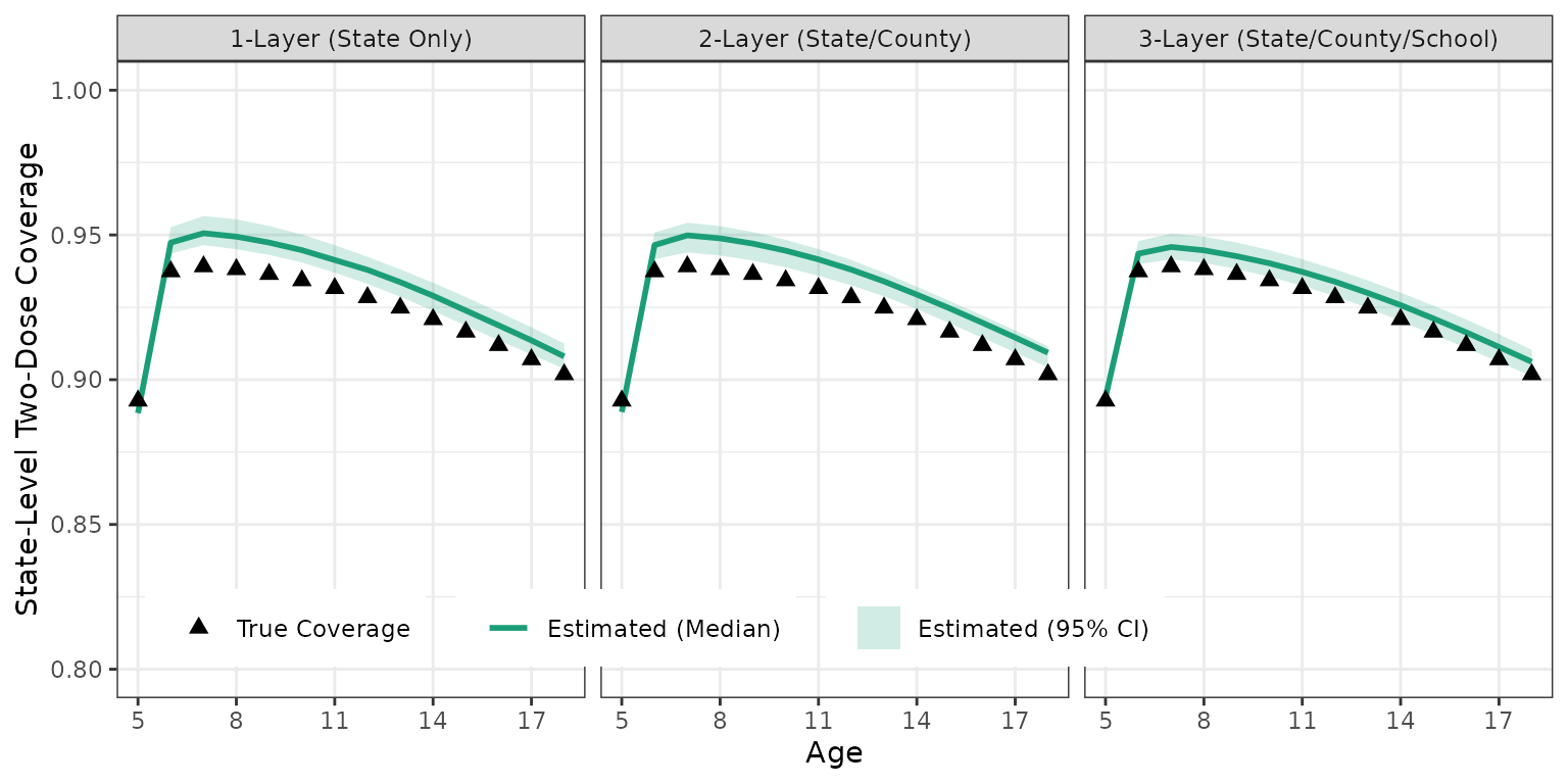
State-level coverage comparison across 1-layer, 2-layer, and 3-layer model fits against true values.
County-Level Coverage Across Data Resolutions
The following plot compares County-level coverage estimates between the 2-layer and 3-layer model fits across counties (Scruggs, Simone, Watson):
Show plot code
counties <- locations_sim[parent_id == state_name, loc_id]

county_2layer_pred <- summary_2layer[
  loc_id %in% counties & dose == 2 & age > 4
][, hierarchy := "2-Layer (State/County)"]
county_3layer_pred <- summary_3layer[
  loc_id %in% counties & dose == 2 & age > 4
][, hierarchy := "3-Layer (State/County/School)"]

county_cov_pred <- rbindlist(list(county_2layer_pred, county_3layer_pred))
h_levels_county <- c("2-Layer (State/County)", "3-Layer (State/County/School)")
county_cov_pred[, hierarchy := factor(hierarchy, levels = h_levels_county)]
county_cov_pred[, loc_id := factor(
  loc_id,
  levels = c("Simone", "Watson", "Scruggs")
)]

county_idx <- predict_sim$target[
  loc_id %in% counties & dose == 2 & age > 4,
  which = TRUE
]
true_county_df <- data.table(
  loc_id = factor(
    predict_sim$target[county_idx, loc_id],
    levels = c("Simone", "Watson", "Scruggs")
  ),
  age = predict_sim$target[county_idx, age],
  coverage = latent_params_sim$coverage[county_idx]
)

true_county_faceted <- rbindlist(lapply(h_levels_county, function(h) {
  df <- copy(true_county_df)
  df[, hierarchy := factor(h, levels = h_levels_county)]
  df
}))

ggplot() +
  geom_ribbon(
    data = county_cov_pred,
    aes(x = age, ymin = q2_5, ymax = q97_5, fill = loc_id),
    alpha = 0.15
  ) +
  geom_line(
    data = county_cov_pred,
    aes(x = age, y = q50, color = loc_id),
    linewidth = 0.9
  ) +
  geom_point(
    data = true_county_faceted,
    aes(x = age, y = coverage, color = loc_id, shape = "True Coverage"),
    size = 2
  ) +
  facet_grid(. ~ hierarchy) +
  scale_shape_manual(name = "", values = c("True Coverage" = 18)) +
  scale_color_discrete(NULL, aesthetics = c("color", "fill")) +
  scale_x_continuous(breaks = seq(5, 18, by = 3), minor_breaks = NULL) +
  coord_cartesian(ylim = c(0.8, 1.0)) +
  theme_bw() +
  theme(
    legend.position = "inside",
    legend.position.inside = c(0.02, 0.05),
    legend.justification.inside = c(0, 0),
    legend.direction = "horizontal",
    legend.box = "horizontal"
  ) +
  labs(
    x = "Age",
    y = "County-Level Two-Dose Coverage"
  )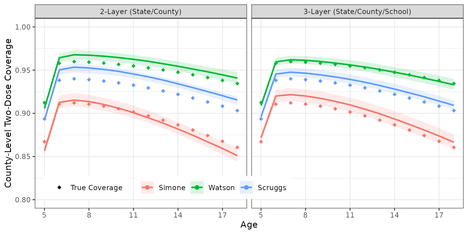
County-level coverage comparison: 2-layer vs. 3-layer model estimates against true values.
Force of Vaccination () Estimation
The following plot shows force of vaccination parameter estimates () across different location data resolutions compared against true values:
Show plot code
extract_lambda_summary <- function(fit, label) {
  draws <- extract_imugap(fit, pars = "lambda_raw")$lambda_raw
  doses_factor <- factor(c(
    rep("Dose 1", nrow(draws)),
    rep("Dose 2", nrow(draws))
  ))
  data.table(
    hierarchy = label,
    dose = doses_factor,
    lambda_raw = c(draws[, 1], draws[, 2])
  )[, .(
    q50 = stats::median(lambda_raw),
    q2_5 = stats::quantile(lambda_raw, 0.025),
    q97_5 = stats::quantile(lambda_raw, 0.975)
  ), by = .(hierarchy, dose)]
}

lambda_est <- rbindlist(list(
  extract_lambda_summary(fit_sim_1layer, "1-Layer"),
  extract_lambda_summary(fit_sim_2layer, "2-Layer"),
  extract_lambda_summary(fit_sim, "3-Layer")
))
h_levels_lambda <- c("1-Layer", "2-Layer", "3-Layer")
lambda_est[, hierarchy := factor(hierarchy, levels = h_levels_lambda)]

true_lambda <- data.table(
  dose = factor(c("Dose 1", "Dose 2")),
  hierarchy = factor("1-Layer", levels = h_levels_lambda),
  true_val = log(latent_params_sim$lambda),
  label = sprintf("True~lambda == %.1f", latent_params_sim$lambda)
)

ggplot(lambda_est, aes(x = hierarchy, y = q50)) +
  geom_hline(
    data = true_lambda,
    aes(yintercept = true_val),
    color = "firebrick",
    linetype = "dashed",
    linewidth = 0.8
  ) +
  geom_label(
    data = true_lambda,
    aes(x = hierarchy, y = true_val, label = label),
    parse = TRUE,
    color = "firebrick",
    fill = ggplot2::alpha("white", 0.75),
    linewidth = NA,
    vjust = -0.3,
    hjust = 0.1,
    size = 3.2
  ) +
  geom_pointrange(
    aes(ymin = q2_5, ymax = q97_5),
    size = 0.7
  ) +
  facet_wrap(~dose) +
  coord_cartesian(ylim = c(0.5, 1.5)) +
  scale_y_continuous(
    transform = "exp",
    labels = function(x) sprintf("%.2f", exp(x))
  ) +
  theme_bw() +
  labs(
    x = "Data Resolution (Model Hierarchy)",
    y = "Uptake Rate (exponential scale)"
  )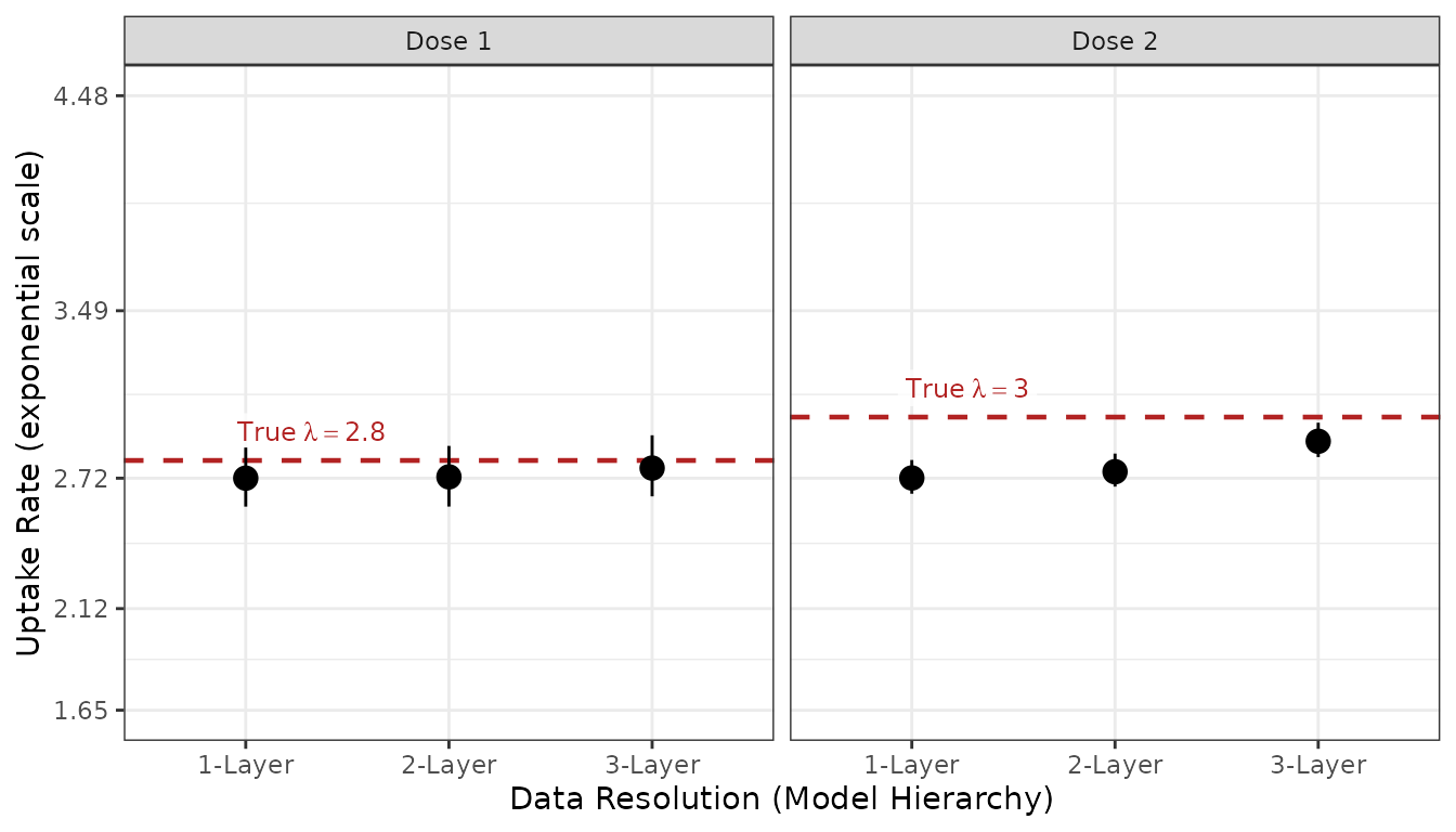
Force of vaccination (lambda) estimates across data resolutions compared to true values.
Conclusion
Support for flexible location layers allows
imuGAP to adapt to whatever population hierarchy you
provide:
- If you provide only state-level aggregated data (1 layer), macro trends are estimated accurately by the process model.
- If you provide sub-populations like counties (2 layers) or sub-sub-populations like schools (3 layers), the model estimates hierarchical random offsets down the tree, allowing you to project cohort trajectories and resolve finer-grained geographic variation.
Summary and Related Vignettes
- For an overview of estimating the underlying process model and predicting coverage, see Getting Started with imuGAP.
- To explore input datasets and validation rules, see Included Example Datasets and Data Validation.
- For convergence diagnostics and trace plots, see Fit Inspection and Stan Diagnostics.