Included Example Datasets and Data Validation

Overview of the Synthetic Simulation Universe

imuGAP provides four bundled datasets (locations_sim, observations_sim, populations_sim, and target_sim) alongside latent parameter fixtures (latent_params_sim, fit_sim, predict_sim) that reflect an underlying vaccination process model and surveillance streams across a multi-resolution hierarchical population structure.

In this scenario:

A single State is partitioned into 3 Counties (Scruggs, Simone, Watson), which contain a total of 24 elementary Schools (10 in Scruggs, 7 in Simone, 7 in Watson).
The vaccine requires a 2-dose sequential regimen (e.g. MMR, with dose 1 recommended at age 1 and dose 2 eligible at age 4).
Observations are gathered from diverse empirical surveillance streams:
- ChildVaxView / NIS-Child: State-level single-cohort point estimates at ages 2 and 3 for dose 1.
- SchoolVaxView: State-level kindergarten entry surveys (dose 2 at age 5).
- TeenVaxView: State-level multi-cohort cross-sectional survey snapshots spanning ages 14 to 18 (dose 2).
- County Sixth-Grade Surveys: Right-censored dose 2 coverage at age 11 across all 3 counties.
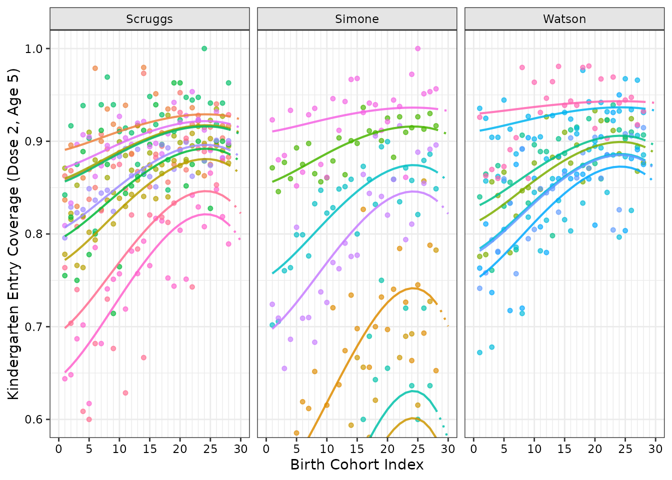
- School Kindergarten Entry Records: Annual kindergarten entry surveys for dose 2 at age 5 across all 24 individual schools.

1. Inspecting the Bundled Datasets

Location Hierarchy (`locations_sim`)

The locations_sim dataset defines the spatial tree structure. Every location node must have either 0 offspring (a leaf node, such as a school) or strictly greater than 1 offspring ( $\ge 2$ children).

data("locations_sim", package = "imuGAP")
head(locations_sim)
#>                  loc_id population parent_id
#>                  <char>      <num>    <char>
#> 1:                State  2895.1333      <NA>
#> 2:              Scruggs  1527.7000     State
#> 3:               Simone   746.6333     State
#> 4:               Watson   620.8000     State
#> 5: Chickadee Elementary   147.8333   Scruggs
#> 6:     Nuthatch Academy   368.5333   Scruggs
nrow(locations_sim)
#> [1] 28

You can validate and canonicalize the location tree using canonicalize_locations():

canonical_locations <- canonicalize_locations(locations_sim)
head(canonical_locations)
#> Key: <layer, parent_id, loc_id>
#>                      loc_id population parent_id layer loc_c_id loc_cp_id
#>                      <char>      <num>    <char> <int>    <int>     <int>
#> 1:                    State 2895.13333      <NA>     1        1        NA
#> 2:                  Scruggs 1527.70000     State     2        2         1
#> 3:                   Simone  746.63333     State     2        3         1
#> 4:                   Watson  620.80000     State     2        4         1
#> 5:        Blue Heron School  115.43333   Scruggs     3        5         2
#> 6: Bluebird Learning Center   49.63333   Scruggs     3        6         2
#>    layer_bound
#>          <int>
#> 1:           1
#> 2:           1
#> 3:           1
#> 4:           1
#> 5:           1
#> 6:           1

canonicalize_locations() introduces:

loc_c_id and loc_cp_id: 1-based integer continuous indices for the location and its parent.
layer: 1-based integer tree depth (1 for State, 2 for County, 3 for School).
layer_bound: Index slicing offsets used internally by Stan to partition the spatial random effect arrays.

Coverage Observations (`observations_sim`)

The observations_sim dataset contains the binomial survey outcomes:

obs_id: Unique identifier for each observation.
loc_id: Location identifier matching a node in locations_sim.
positive: Count of vaccinated individuals.
sample_n: Total sample size ( $N$ ).
censored: 1 for right-censored observations, NA for uncensored observations.

data("observations_sim", package = "imuGAP")
head(observations_sim[, .(obs_id, loc_id, positive, sample_n, censored)])
#>    obs_id               loc_id positive sample_n censored
#>     <int>               <char>    <num>    <int>    <num>
#> 1:      1 Chickadee Elementary      135      155       NA
#> 2:      2 Chickadee Elementary      124      152       NA
#> 3:      3 Chickadee Elementary      133      156       NA
#> 4:      4 Chickadee Elementary      127      155       NA
#> 5:      5 Chickadee Elementary      141      155       NA
#> 6:      6 Chickadee Elementary      139      158       NA

Canonicalizing observations with canonicalize_observations() assigns continuous 1-based indices obs_c_id, sorting uncensored records before censored records for efficient block execution in Stan:

canonical_observations <- canonicalize_observations(observations_sim)
head(canonical_observations)
#> Key: <censored, obs_id>
#>    obs_c_id positive sample_n censored obs_id
#>       <int>    <int>    <int>    <num>  <int>
#> 1:        1      135      155       NA      1
#> 2:        2      124      152       NA      2
#> 3:        3      133      156       NA      3
#> 4:        4      127      155       NA      4
#> 5:        5      141      155       NA      5
#> 6:        6      139      158       NA      6

Observation Metadata & Populations (`populations_sim`)

The populations table provides essential metadata for all observations—defining the discrete location, age, cohort, and dose associated with each survey outcome. Every record in observations receives one or more entries in populations:

Direct (1:1) observations: A single row with weight = 1.0 maps the observation directly to a discrete population slice (such as a single-cohort kindergarten survey at age 5).
Mixed observations: When a survey mixes multiple underlying populations (such as cross-sectional surveys spanning multiple age groups or cohorts), populations captures this mixture using multiple rows sharing the same obs_id, each assigned a fractional weight (e.g. equal weights or demographic population shares summing to 1.0).

data("populations_sim", package = "imuGAP")
head(populations_sim)
#>    obs_id               loc_id cohort   age  dose weight
#>     <int>               <char>  <int> <int> <int>  <num>
#> 1:      1 Chickadee Elementary      1     5     2      1
#> 2:      2 Chickadee Elementary      2     5     2      1
#> 3:      3 Chickadee Elementary      3     5     2      1
#> 4:      4 Chickadee Elementary      4     5     2      1
#> 5:      5 Chickadee Elementary      5     5     2      1
#> 6:      6 Chickadee Elementary      6     5     2      1

For single-cohort kindergarten surveys, obs_id has a 1:1 mapping with weight = 1.0. For multi-age surveys (such as TeenVaxView at obs_id == 761), multiple rows describe the mixture across ages:

# TeenVaxView-style observation spanning ages 14 to 18
observations_sim[
  obs_id == 761,
  .(obs_id, loc_id, positive, sample_n, age_min, age_max, dose)
]
#>    obs_id loc_id positive sample_n age_min age_max  dose
#>     <int> <char>    <num>    <int>   <int>   <int> <int>
#> 1:    761  State      217      250      14      19     2

# Corresponding population metadata with distributed weights summing to 1.0
populations_sim[obs_id == 761]
#>    obs_id loc_id cohort   age  dose weight
#>     <int> <char>  <int> <int> <int>  <num>
#> 1:    761  State      5    14     2    0.2
#> 2:    761  State      4    15     2    0.2
#> 3:    761  State      3    16     2    0.2
#> 4:    761  State      2    17     2    0.2
#> 5:    761  State      1    18     2    0.2

You can validate and canonicalize populations using canonicalize_populations():

canonical_populations <- canonicalize_populations(
  populations_sim, observations_sim, locations_sim
)
head(canonical_populations)
#> Key: <obs_c_id, loc_c_id, cohort, age, dose>
#>    obs_id               loc_id cohort   age  dose weight obs_c_id loc_c_id
#>     <int>               <char>  <int> <int> <int>  <num>    <int>    <int>
#> 1:      1 Chickadee Elementary      1     5     2      1        1        8
#> 2:      2 Chickadee Elementary      2     5     2      1        2        8
#> 3:      3 Chickadee Elementary      3     5     2      1        3        8
#> 4:      4 Chickadee Elementary      4     5     2      1        4        8
#> 5:      5 Chickadee Elementary      5     5     2      1        5        8
#> 6:      6 Chickadee Elementary      6     5     2      1        6        8
#>    range_start
#>          <int>
#> 1:           1
#> 2:           2
#> 3:           3
#> 4:           4
#> 5:           5
#> 6:           6

2. Canonicalization Rules and Validation Diagnostics

imuGAP enforces strict structural assertions to safeguard model fitting against corrupted or incompatible inputs:

Observation Binomial Count Consistency

If an observation has positive > sample_n, canonicalize_observations() raises an informative error:

invalid_obs <- copy(observations_sim[, .(obs_id, loc_id, positive, sample_n, censored)])
invalid_obs[1, positive := sample_n + 10]

tryCatch(
  canonicalize_observations(invalid_obs),
  error = function(e) message("Caught expected error: ", e$message)
)
#> Caught expected error: `observations` column 'positive' must be <= 'sample_n'; found 1 invalid row(s) with obs_id: 1; use `subset(observations, positive > sample_n)` to resolve invalid entries

Hierarchy Invariant Enforcement

If duplicate location IDs exist, or single-child chains are introduced, canonicalize_locations() rejects the tree:

invalid_locs <- rbind(
  locations_sim,
  data.frame(loc_id = "Scruggs", parent_id = "State"),
  fill = TRUE
)

tryCatch(
  canonicalize_locations(invalid_locs),
  error = function(e) message("Caught expected error: ", e$message)
)
#> Caught expected error: `locations` column 'loc_id' must contain unique values; found 1 duplicate(s): Scruggs; use `subset(locations, duplicated(loc_id) | duplicated(loc_id, fromLast = TRUE))` to resolve invalid entries

3. Visualizing the Synthetic Observation Streams

The following figures illustrate empirical coverage rates across each observation stream compared against underlying true data-generating parameters (latent_params_sim).

State-Level Observation Streams

Show plot code

data("latent_params_sim", package = "imuGAP")

state_obs <- copy(observations_sim[loc_id == "State"])
state_obs[, source := factor(
  fcase(
    dose == 1 & age_min == 2, "ChildVaxView (Dose 1, Age 2)",
    dose == 1 & age_min == 3, "ChildVaxView (Dose 1, Age 3)",
    age_min == 5, "SchoolVaxView (Dose 2, Age 5)",
    default = "TeenVaxView (Dose 2, Ages 14-18)"
  ),
  levels = c(
    "ChildVaxView (Dose 1, Age 2)",
    "ChildVaxView (Dose 1, Age 3)",
    "SchoolVaxView (Dose 2, Age 5)",
    "TeenVaxView (Dose 2, Ages 14-18)"
  )
)]
state_obs[, obs_prop := positive / sample_n]

single_cohort_obs <- state_obs[is.na(age_max) | age_max == age_min + 1L]
multi_cohort_obs <- copy(state_obs[!is.na(age_max) & age_max > age_min + 1L])
multi_cohort_obs[, cohort_max := cohort_min + (age_max - 1L) - age_min]

latent_state <- data.table(
  cohort_min = seq_along(latent_params_sim$phi_state),
  propensity = 1 - latent_params_sim$phi_state
)

n_c <- length(latent_params_sim$phi_state)
skv_max_cohort <- max(state_obs[age_min == 5, cohort_min])
tvv_max_cohort <- max(multi_cohort_obs$cohort_min)

latent_curves <- rbindlist(list(
  data.table(
    cohort_min = seq_len(n_c),
    latent_cov = (1 - latent_params_sim$phi_state) *
      latent_params_sim$uptake[2, 1],
    source = "ChildVaxView (Dose 1, Age 2)"
  ),
  data.table(
    cohort_min = seq_len(n_c),
    latent_cov = (1 - latent_params_sim$phi_state) *
      latent_params_sim$uptake[3, 1],
    source = "ChildVaxView (Dose 1, Age 3)"
  ),
  data.table(
    cohort_min = seq_len(skv_max_cohort),
    latent_cov = (1 - latent_params_sim$phi_state[seq_len(skv_max_cohort)]) *
      latent_params_sim$uptake[5, 2],
    source = "SchoolVaxView (Dose 2, Age 5)"
  ),
  data.table(
    cohort_min = seq_len(tvv_max_cohort),
    latent_cov = (1 - latent_params_sim$phi_state[seq_len(tvv_max_cohort)]) *
      mean(latent_params_sim$uptake[14:18, 2]),
    source = "TeenVaxView (Dose 2, Ages 14-18)"
  )
))
latent_curves[, source := factor(source, levels = levels(state_obs$source))]

ggplot() +
  geom_line(
    data = latent_state,
    aes(x = cohort_min, y = propensity, linetype = "True Lifetime Uptake Propensity (1 - phi)"),
    color = "gray40", linewidth = 0.8, alpha = 0.5
  ) +
  geom_line(
    data = latent_curves,
    aes(x = cohort_min, y = latent_cov, color = source),
    linetype = "dashed", linewidth = 0.7, alpha = 0.4
  ) +
  geom_segment(
    data = multi_cohort_obs,
    aes(x = cohort_min, xend = cohort_max, y = obs_prop, yend = obs_prop, color = source),
    linewidth = 1.1, alpha = 0.95
  ) +
  geom_point(
    data = single_cohort_obs,
    aes(x = cohort_min, y = obs_prop, color = source, shape = source),
    size = 2.4, alpha = 0.95
  ) +
  scale_x_continuous(breaks = seq(0, 30, by = 5), minor_breaks = seq(1, 30, by = 1)) +
  coord_cartesian(xlim = c(0, 30), ylim = c(0.4, 1.0)) +
  scale_linetype_manual(
    name = NULL,
    values = c("True Lifetime Uptake Propensity (1 - phi)" = "dashed")
  ) +
  scale_color_brewer(name = "Data Source", palette = "Dark2") +
  scale_shape_manual(
    name = "Data Source",
    values = c(
      "ChildVaxView (Dose 1, Age 2)" = 16,
      "ChildVaxView (Dose 1, Age 3)" = 17,
      "SchoolVaxView (Dose 2, Age 5)" = 15,
      "TeenVaxView (Dose 2, Ages 14-18)" = 18
    )
  ) +
  guides(
    color = guide_legend(
      override.aes = list(
        shape = c(16, 17, 15, NA),
        linetype = c("blank", "blank", "blank", "solid"),
        linewidth = c(0, 0, 0, 1.1),
        alpha = 1
      )
    ),
    shape = "none"
  ) +
  theme(
    legend.position = "inside",
    legend.position.inside = c(0.98, 0.02),
    legend.justification.inside = c(1, 0)
  ) +
  labs(x = "Birth Cohort Index", y = "Vaccination Proportion")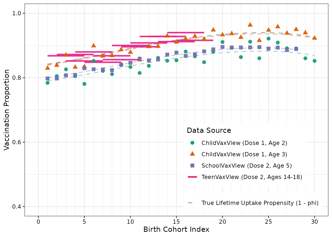

County-Level Right-Censored Surveillance

imuGAP supports observations at intermediate spatial resolutions as well as right-censored surveillance streams.

In public health surveillance, records often report composite vaccine series completion (for example, whether a student has received all required middle school entry immunizations) rather than tracking a specific vaccine in isolation. Because an individual who completed the full multi-vaccine series has necessarily received the target vaccine, the observed series completion rate acts as a lower bound on the target vaccine’s true coverage (true coverage $\ge$ observed proportion).

imuGAP natively models right-censored observations:

In observations, you mark right-censored survey records with censored = 1 (and uncensored records with NA).
During Bayesian model fitting, the likelihood accounts for the right-censoring mechanism, ensuring that lower-bound surveillance records accurately inform the latent process without biasing coverage trajectories downward.

In this simulation universe, routine county-wide middle school entry tallies (dose 2 at age 11) across all three counties represent right-censored surveillance streams:

Show plot code

county_names <- names(latent_params_sim$off_cnty)
county_obs <- copy(observations_sim[loc_id %in% county_names])
county_obs[, obs_prop := positive / sample_n]

max_obs_cohort <- max(county_obs$cohort_min)
n_cohorts <- length(latent_params_sim$phi_state)

county_latent <- rbindlist(lapply(names(latent_params_sim$off_cnty), function(cnty) {
  cohorts <- seq_len(n_cohorts)
  c_idx <- match(cnty, names(latent_params_sim$off_cnty))
  offset <- latent_params_sim$off_cnty[c_idx]
  phi_shifted <- plogis(qlogis(latent_params_sim$phi_state[cohorts]) + offset)
  cov_true <- (1 - phi_shifted) * latent_params_sim$uptake[11, 2]
  cov_censored <- cov_true * latent_params_sim$censor_reduction
  data.table(
    loc_id = cnty,
    cohort_min = cohorts,
    latent_cov = cov_true,
    latent_cov_censored = cov_censored
  )
}))

county_latent_obs <- county_latent[cohort_min <= max_obs_cohort]
county_latent_unobs <- county_latent[cohort_min >= max_obs_cohort]

ggplot() +
  geom_point(
    data = county_obs,
    aes(x = cohort_min, y = obs_prop),
    color = "steelblue", size = 2, alpha = 0.85
  ) +
  geom_line(
    data = county_latent_obs,
    aes(
      x = cohort_min,
      y = latent_cov,
      color = "True Latent Coverage",
      linetype = "Observed Cohorts"
    ),
    linewidth = 0.9
  ) +
  geom_line(
    data = county_latent_obs,
    aes(
      x = cohort_min,
      y = latent_cov_censored,
      color = "Censored Latent (0.95x)",
      linetype = "Observed Cohorts"
    ),
    linewidth = 0.9
  ) +
  geom_line(
    data = county_latent_unobs,
    aes(
      x = cohort_min,
      y = latent_cov,
      color = "True Latent Coverage",
      linetype = "Unobserved Cohorts"
    ),
    linewidth = 0.9
  ) +
  geom_line(
    data = county_latent_unobs,
    aes(
      x = cohort_min,
      y = latent_cov_censored,
      color = "Censored Latent (0.95x)",
      linetype = "Unobserved Cohorts"
    ),
    linewidth = 0.9
  ) +
  facet_wrap(~loc_id) +
  scale_x_continuous(breaks = seq(0, 30, by = 5), minor_breaks = seq(1, 30, by = 1)) +
  scale_y_continuous(expand = c(0, 0)) +
  coord_cartesian(xlim = c(0, 30), ylim = c(0.6, 1.0)) +
  scale_color_manual(
    name = NULL,
    values = c("True Latent Coverage" = "firebrick", "Censored Latent (0.95x)" = "darkorange")
  ) +
  scale_linetype_manual(
    name = NULL,
    values = c("Observed Cohorts" = "dashed", "Unobserved Cohorts" = "dotted")
  ) +
  guides(
    color = guide_legend(order = 1, override.aes = list(linewidth = 0.9, linetype = "solid")),
    linetype = guide_legend(order = 2, override.aes = list(linewidth = 0.9, color = "black"))
  ) +
  theme(
    legend.position = "inside",
    legend.position.inside = c(0.85, 0.12),
    legend.justification.inside = c(1, 0)
  ) +
  labs(x = "Birth Cohort Index", y = "6th Grade Survey Coverage (Dose 2, Age 11)")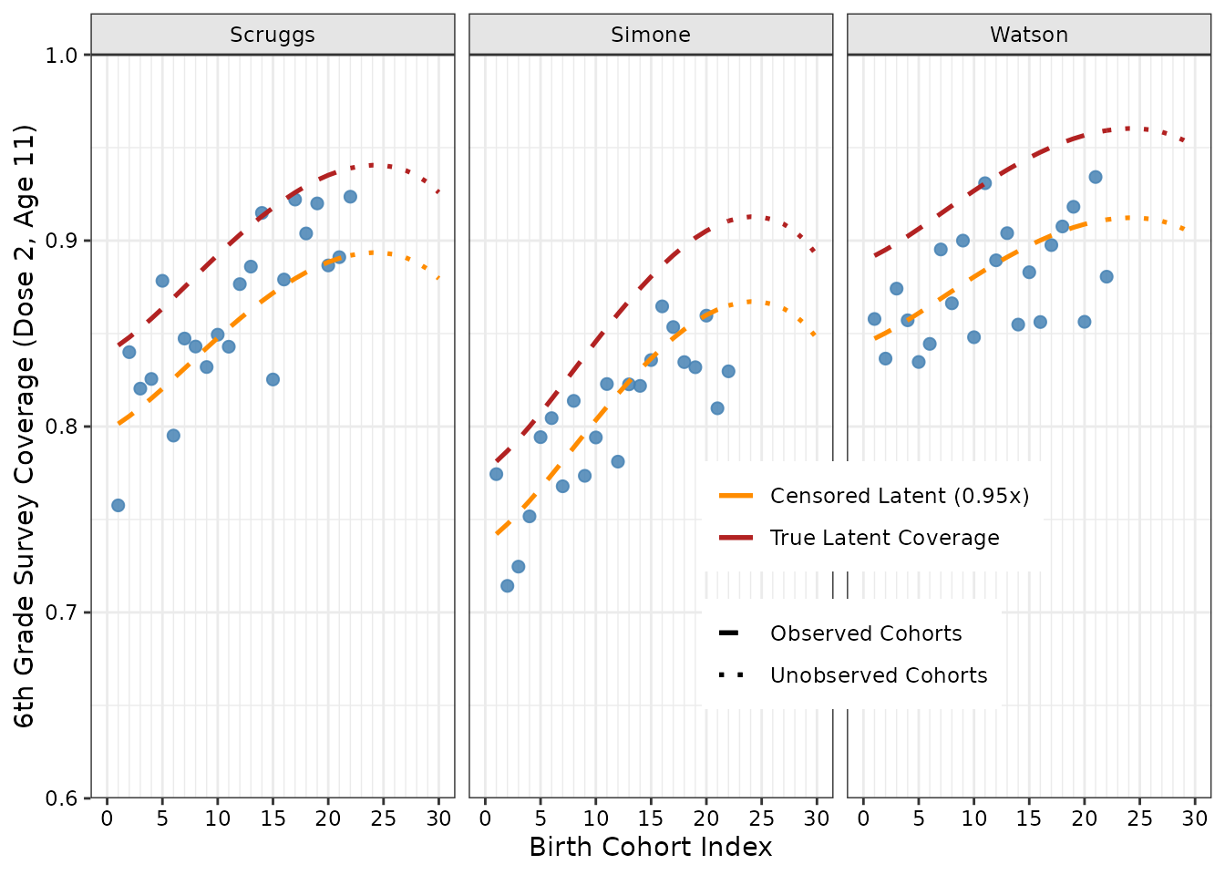

School Kindergarten Enrollment Records

The following plot illustrates school-level kindergarten entry records (dose 2 at age 5) across all elementary schools grouped by county, comparing empirical survey counts against the underlying school-specific latent coverage curves:

Show plot code

canonical_locations <- canonicalize_locations(locations_sim)
sch_locs <- canonical_locations[layer == 3]

n_cohorts <- length(latent_params_sim$phi_state)
off_c <- latent_params_sim$off_cnty
off_s <- latent_params_sim$off_sch
uptake_val <- latent_params_sim$uptake[5, 2]

school_latent <- rbindlist(lapply(seq_len(nrow(sch_locs)), function(i) {
  sch <- sch_locs$loc_id[i]
  cnty <- sch_locs$parent_id[i]
  tot_off <- unname(off_c[cnty]) + unname(off_s[sch])
  cohorts <- seq_len(n_cohorts)
  phi_shifted <- plogis(qlogis(latent_params_sim$phi_state[cohorts]) + tot_off)
  cov_true <- (1 - phi_shifted) * uptake_val
  data.table(loc_id = sch, county_id = cnty, cohort_min = cohorts, latent_cov = cov_true)
}))

sch_obs <- copy(observations_sim[loc_id %in% sch_locs$loc_id])
sch_obs[, obs_prop := positive / sample_n]
sch_obs <- merge(sch_obs, sch_locs[, .(loc_id, county_id = parent_id)], by = "loc_id")

max_obs_cohort <- max(sch_obs$cohort_min)
school_latent_obs <- school_latent[cohort_min <= max_obs_cohort]
school_latent_unobs <- school_latent[cohort_min >= max_obs_cohort]

ggplot() +
  geom_point(
    data = sch_obs,
    aes(x = cohort_min, y = obs_prop, color = loc_id),
    size = 1.3, alpha = 0.65
  ) +
  geom_line(
    data = school_latent_obs,
    aes(
      x = cohort_min,
      y = latent_cov,
      group = loc_id,
      color = loc_id,
      linetype = "Observed Cohorts"
    ),
    linewidth = 0.75, alpha = 0.85
  ) +
  geom_line(
    data = school_latent_unobs,
    aes(
      x = cohort_min,
      y = latent_cov,
      group = loc_id,
      color = loc_id,
      linetype = "Unobserved Cohorts"
    ),
    linewidth = 0.75, alpha = 0.85
  ) +
  facet_wrap(~county_id) +
  scale_x_continuous(breaks = seq(0, 30, by = 5), minor_breaks = seq(1, 30, by = 1)) +
  coord_cartesian(xlim = c(0, 30), ylim = c(0.6, 1.0)) +
  scale_linetype_manual(
    name = NULL,
    values = c("Observed Cohorts" = "solid", "Unobserved Cohorts" = "dotted")
  ) +
  theme(legend.position = "none") +
  labs(
    x = "Birth Cohort Index",
    y = "Kindergarten Entry Coverage (Dose 2, Age 5)"
  )

For an overview of estimating the underlying process model and predicting coverage, see Getting Started with imuGAP.
To learn how imuGAP configures and estimates parameters across arbitrary spatial depths, see Flexible Location Layers in imuGAP.
For detailed MCMC convergence checks, trace plots, and parameter inference, see Fit Inspection and Stan Diagnostics.

Overview of the Synthetic Simulation Universe

1. Inspecting the Bundled Datasets

Location Hierarchy (locations_sim)

Coverage Observations (observations_sim)

Observation Metadata & Populations (populations_sim)

2. Canonicalization Rules and Validation Diagnostics

Observation Binomial Count Consistency

Hierarchy Invariant Enforcement

3. Visualizing the Synthetic Observation Streams

State-Level Observation Streams

County-Level Right-Censored Surveillance

School Kindergarten Enrollment Records

Summary and Related Vignettes

Location Hierarchy (`locations_sim`)

Coverage Observations (`observations_sim`)

Observation Metadata & Populations (`populations_sim`)