Introduction
The name imuGAP stands for “Immunity: Geographic &
Age-based Projection”. This package allows the user to synthesize across
multiple data sources to make predictions of vaccination coverage for
user-defined populations of interest. For example, one could use the
package to:
- Estimate current vaccination coverage by location across different age groups
- Estimate coverage (or uptake) for a given birth cohort (e.g. people born in 1990) across their life course (i.e. at each age from birth to current age)
- Fill in gaps in observed coverage data (e.g. a school that doesn’t report vaccination coverage in a certain year)
More specifically, the package provides a stan-based model for estimating vaccination coverage by location, cohort, and age for childhood infectious diseases, such as measles. The core model represents a target population as having a life-long propensity for vaccination; some proportion, , of that population is unlikely to vaccinate and the complementary proportion, , is likely to vaccinate. That population then experiences a vaccination rate, , over the model time eras, according to the vaccination eligibility schedule, . These core parameters can vary over time and location, in a user-specifiable way.
Focusing just on the core model element, imagine a particular population location and cohort (where denotes the start of the time period when that group was born). If that cohort is now age , and the vaccine schedule for the first dose is , the expected fraction of that group to have at least one dose is then:
Which is to say, we are representing vaccination coverage via a survival-like model. The model generalizes this approach to the first dose out to arbitrary sequential dose coverage, with each subsequent dose conditional on previous dose receipt.
Walkthrough of Basic Usage
This walkthrough demonstrates the workflow of fitting the model and predicting coverage on simulated data. The package includes several bundled datasets for demonstration, representing a nested geographic hierarchy (State -> Counties -> Schools) for population uptake of a two dose vaccine, like MMR for measles.
1. Preparing and Validating the Input Data
First, let’s explore the three required inputs that define the
location hierarchy, observation metadata, and the actual coverage
observations. The package provides a family of
canonicalize_* functions to validate, clean, and convert
these raw structures into the canonical forms required by the sampler.
You can use those directly to help troubleshoot your inputs, as we do in
the following examples. However, as shown in the next section, the
sampling() method also automatically canonicalizes the
inputs.
Location Hierarchy (locations_sim)
The locations dataset defines the nesting relationship of the
locations in the model. In this simulation, we have a State, which
contains three Counties, which in turn contain various Schools. We
validate and canonicalize it using
canonicalize_locations().
data("locations_sim", package = "imuGAP")
head(locations_sim)
#>                  loc_id parent_id
#>                  <char>    <char>
#> 1:                State      <NA>
#> 2:              Scruggs     State
#> 3:               Simone     State
#> 4:               Watson     State
#> 5: Chickadee Elementary   Scruggs
#> 6:     Nuthatch Academy   Scruggs

# Canonicalize and validate
canonical_locations <- canonicalize_locations(locations_sim)
head(canonical_locations)
#> Key: <layer, parent_id, loc_id>
#>                      loc_id parent_id layer loc_c_id loc_cp_id layer_bound
#>                      <char>    <char> <int>    <int>     <int>       <int>
#> 1:                    State      <NA>     1        1        NA           1
#> 2:                  Scruggs     State     2        2         1           1
#> 3:                   Simone     State     2        3         1           1
#> 4:                   Watson     State     2        4         1           1
#> 5:        Blue Heron School   Scruggs     3        5         2           1
#> 6: Bluebird Learning Center   Scruggs     3        6         2           1
Coverage Observations (observations_sim)
The observations dataset contains the counts of individuals who were
vaccinated (positive) out of the total sampled
(sample_n) for each observation. It also includes a
censored column, which is 1 if the observation
is right-censored and NA otherwise. We validate and
canonicalize it using canonicalize_observations().
data("observations_sim", package = "imuGAP")
head(observations_sim[, .(obs_id, loc_id, positive, sample_n, censored)])
#>    obs_id               loc_id positive sample_n censored
#>     <int>               <char>    <num>    <num>    <num>
#> 1:      1 Chickadee Elementary       16       19       NA
#> 2:      2 Chickadee Elementary       14       20       NA
#> 3:      3 Chickadee Elementary       14       16       NA
#> 4:      4 Chickadee Elementary       10       13       NA
#> 5:      5 Chickadee Elementary        8       13       NA
#> 6:      6 Chickadee Elementary        7        8       NA

# Canonicalize and validate
canonical_observations <- canonicalize_observations(observations_sim)
head(canonical_observations)
#> Key: <censored, obs_id>
#>    obs_c_id positive sample_n censored obs_id
#>       <int>    <int>    <int>    <num>  <int>
#> 1:        1       16       19       NA      1
#> 2:        2       14       20       NA      2
#> 3:        3       14       16       NA      3
#> 4:        4       10       13       NA      4
#> 5:        5        8       13       NA      5
#> 6:        6        7        8       NA      6
Observation Metadata (populations_sim)
The populations dataset acts as observation metadata, mapping each
observation ID (obs_id) to the corresponding location,
birth cohort, age at observation, vaccine dose, and observation weight.
We validate and canonicalize it using
canonicalize_populations().
data("populations_sim", package = "imuGAP")
head(populations_sim)
#>    obs_id               loc_id cohort   age  dose weight
#>     <num>               <char>  <num> <num> <num>  <num>
#> 1:      1 Chickadee Elementary      4     5     2      1
#> 2:      2 Chickadee Elementary      5     5     2      1
#> 3:      3 Chickadee Elementary      6     5     2      1
#> 4:      4 Chickadee Elementary      7     5     2      1
#> 5:      5 Chickadee Elementary      8     5     2      1
#> 6:      6 Chickadee Elementary      9     5     2      1

# Canonicalize and validate
canonical_populations <- canonicalize_populations(
  populations_sim, observations_sim, locations_sim
)
head(canonical_populations)
#> Key: <obs_c_id, loc_c_id, cohort, age, dose>
#>    obs_id               loc_id cohort   age  dose weight obs_c_id loc_c_id
#>     <num>               <char>  <int> <int> <num>  <num>    <int>    <int>
#> 1:      1 Chickadee Elementary      4     5     2      1        1        8
#> 2:      2 Chickadee Elementary      5     5     2      1        2        8
#> 3:      3 Chickadee Elementary      6     5     2      1        3        8
#> 4:      4 Chickadee Elementary      7     5     2      1        4        8
#> 5:      5 Chickadee Elementary      8     5     2      1        5        8
#> 6:      6 Chickadee Elementary      9     5     2      1        6        8
#>    range_start
#>          <int>
#> 1:           1
#> 2:           2
#> 3:           3
#> 4:           4
#> 5:           5
#> 6:           6
Validation Failure Examples
To ensure data integrity, the canonicalize_* functions
enforce strict rules on the input data format and constraints. For
example, if we modify the observations data so that the number of
positive cases exceeds the total sample size
sample_n, the validation function will raise a clear
error:
# Create a copy with an invalid observation (positive > sample_n)
invalid_obs <- copy(observations_sim[, .(obs_id, loc_id, positive, sample_n, censored)])
invalid_obs[1, positive := sample_n + 10]

# This will fail validation and throw an error:
tryCatch(
  canonicalize_observations(invalid_obs),
  error = function(e) message("Caught expected error: ", e$message)
)
#> Caught expected error: positive must be <= sample_n; found 1 invalid observations with offending ids: 1
Similarly, if the locations data contains duplicate location IDs,
canonicalize_locations() will detect the duplication and
throw an error:
# Create a copy with a duplicate location ID
invalid_locs <- rbind(
  locations_sim,
  data.frame(loc_id = "Scruggs", parent_id = "State")
)

# This will fail validation:
tryCatch(
  canonicalize_locations(invalid_locs),
  error = function(e) message("Caught expected error: ", e$message)
)
#> Caught expected error: locations$loc_id must be unique; found 1 duplicates: 29
See the canonicalize_* function documentation for more
complete validation requirements.
2. Fitting the Model
Using the prepared input datasets, we can fit the Bayesian model
using sampling(). The options for the sampler can be
configured using stan_options().
Because compiling the Stan model and running the MCMC chain can take some time, we show the code below without executing it.
fit_sim <- sampling(
  observations_sim, populations_sim, locations_sim,
  stan_opts = stan_options(
    iter = 2000, chains = 4, refresh = 0, seed = 1L
  )
)
For this walkthrough, we load the pre-computed fit object
fit_sim bundled with the package:
data("fit_sim", package = "imuGAP")Once the model is fit, we can extract posterior draws of the model
parameters using extract_imugap(). For example, let’s
extract the B-spline coefficients representing the state-level vaccine
uptake baseline:
beta_draws <- extract_imugap(fit_sim, pars = "beta_bs")
str(beta_draws)
#> List of 1
#>  $ beta_bs: num [1:2000, 1:5] -1.71 -1.59 -1.84 -1.84 -1.69 ...
#>   ..- attr(*, "dimnames")=List of 2
#>   .. ..$ iterations: NULL
#>   .. ..$           : NULL
We can also look at trace plots for selected parameters to ensure convergence has been reached.
bayesplot::mcmc_trace(fit_sim$stanfit,
  pars = c(
    "beta_bs[1]", "beta_bs[2]", "beta_bs[3]",
    "beta_bs[4]", "beta_bs[5]"
  )
) + theme_bw() +
  theme(legend.position = c(.9, .1), legend.justification = c(1, 0))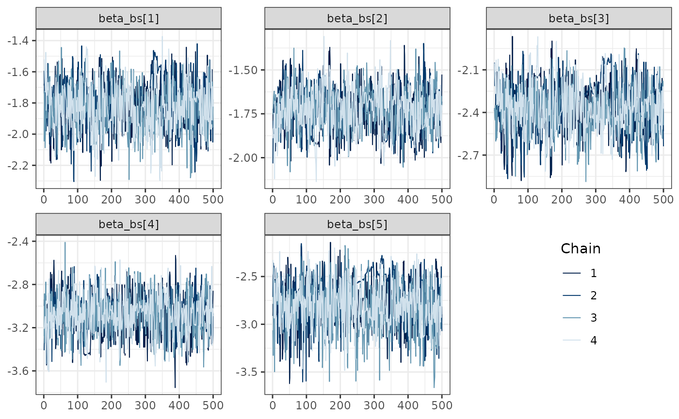
3. Defining a Target for Predictions
To predict vaccine coverage for a target population (which can
include locations or cohorts without direct observations, as long as
they exist in the locations hierarchy), we first define a target grid
using create_target(). Note that predictions can only be
made for birth cohorts and locations that have at least some
observations included in the estimation run. In other words, the model
cannot predict coverage for future birth cohorts or unobserved
locations.
For example, we can generate a “snapshot” prediction target for all locations, including the State and County levels, across ages 1 to 18:
target_sim <- create_target(
  fit = fit_sim, location = unique(locations_sim$loc_id), age = 1:18,
  cohort = max(populations_sim$cohort) - 18, dose = c(1, 2), mode = "snapshot"
)
head(target_sim)
#>    obs_c_id               loc_id   age cohort  dose weight loc_c_id
#>       <int>               <char> <int>  <num> <num>  <num>    <int>
#> 1:        1                State     1     30     1      1        1
#> 2:        2              Scruggs     1     30     1      1        2
#> 3:        3               Simone     1     30     1      1        3
#> 4:        4               Watson     1     30     1      1        4
#> 5:        5 Chickadee Elementary     1     30     1      1        8
#> 6:        6     Nuthatch Academy     1     30     1      1       11
4. Predicting Coverage
Finally, we run predict() to generate predicted coverage
probabilities for each target population combination. By default it uses
every posterior draw; here we pass posterior_size to
predict over a smaller sub-sample taken from the end of each chain.
Generating predictions also runs the Stan model (in generated quantities mode) and can be time-consuming, so we show the code below without executing it:
predict_sim <- predict(object = fit_sim, target = target_sim, posterior_size = 100)Instead, we load the pre-computed prediction results
predict_sim bundled with the package. This is an object of
class imugap_predict which contains a 3D draws array
(predict_sim$draws) with the MCMC draws for each prediction
target as well as the target information
(predict_sim$target).
data("predict_sim", package = "imuGAP")We can summarize these predictions to get the posterior mean and credible intervals across the target location, age, and doses requested:
# Calculate the posterior mean coverage probability for each location and dose at age 5
summary_predict <- summary(predict_sim)
head(summary_predict)
#>    obs_c_id               loc_id   age cohort  dose weight loc_c_id obs_id
#>       <int>               <char> <int>  <num> <num>  <num>    <int>  <int>
#> 1:        1                State     1     30     1      1        1      1
#> 2:        2              Scruggs     1     30     1      1        2      2
#> 3:        3               Simone     1     30     1      1        3      3
#> 4:        4               Watson     1     30     1      1        4      4
#> 5:        5 Chickadee Elementary     1     30     1      1        8      5
#> 6:        6     Nuthatch Academy     1     30     1      1       11      6
#>     mean  q2_5   q50 q97_5
#>    <num> <num> <num> <num>
#> 1:     0     0     0     0
#> 2:     0     0     0     0
#> 3:     0     0     0     0
#> 4:     0     0     0     0
#> 5:     0     0     0     0
#> 6:     0     0     0     0
Now let’s visualize the results. First we will take a look at overall state coverage by cohort. Note that the lower coverage among 5 year olds is due to them only having been eligible for their second dose for one year.
summary_predict |>
  subset(loc_id == "State" & dose == 2 & age > 4) |>
  ggplot() +
  aes(x = age) +
  geom_line(aes(y = q50)) +
  geom_ribbon(aes(ymin = q2_5, ymax = q97_5), alpha = 0.5) +
  theme_bw() +
  scale_x_continuous(breaks = 5:18, minor_breaks = NULL) +
  labs(x = "Age", y = "Coverage", title = "State-level two dose coverage")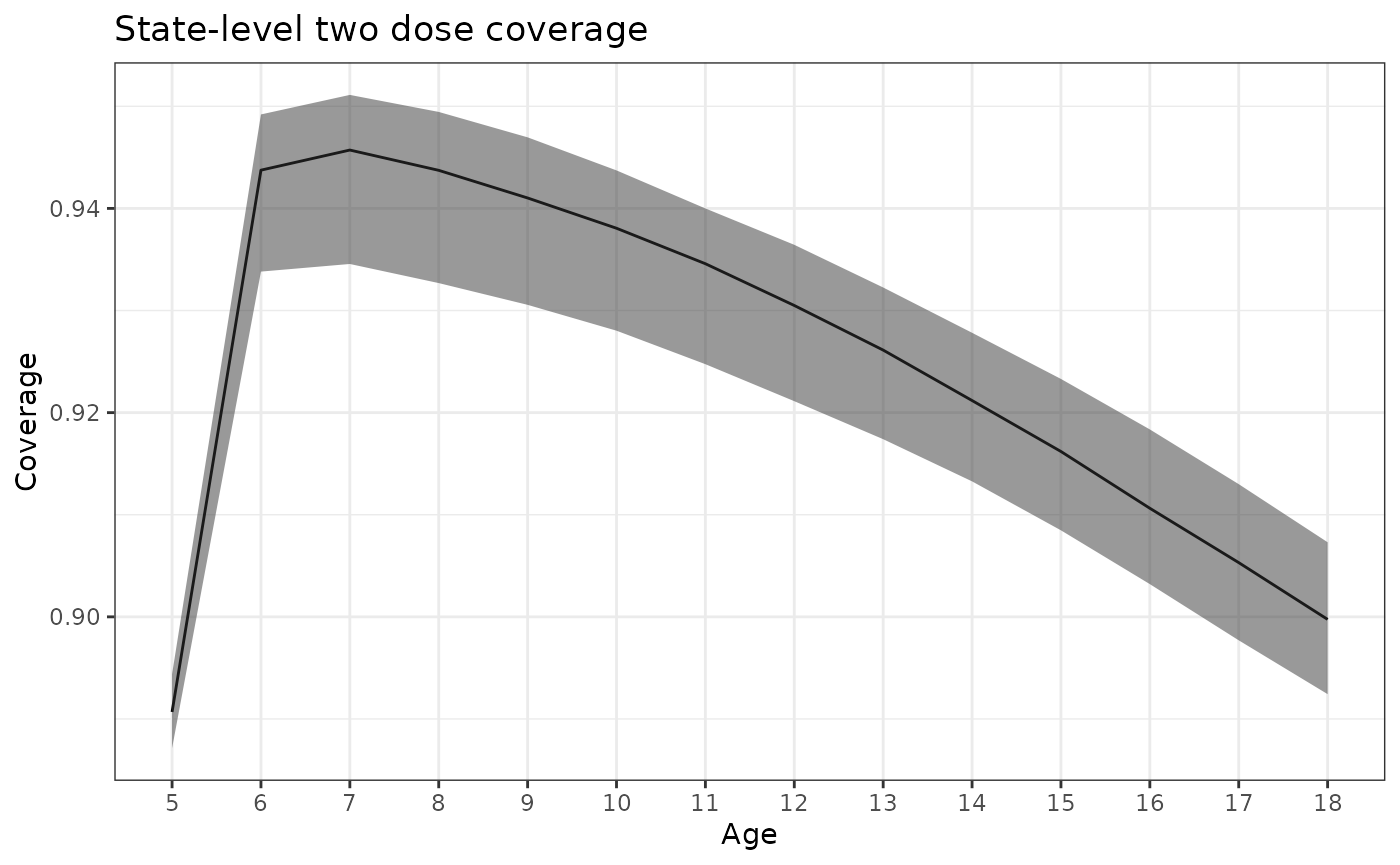
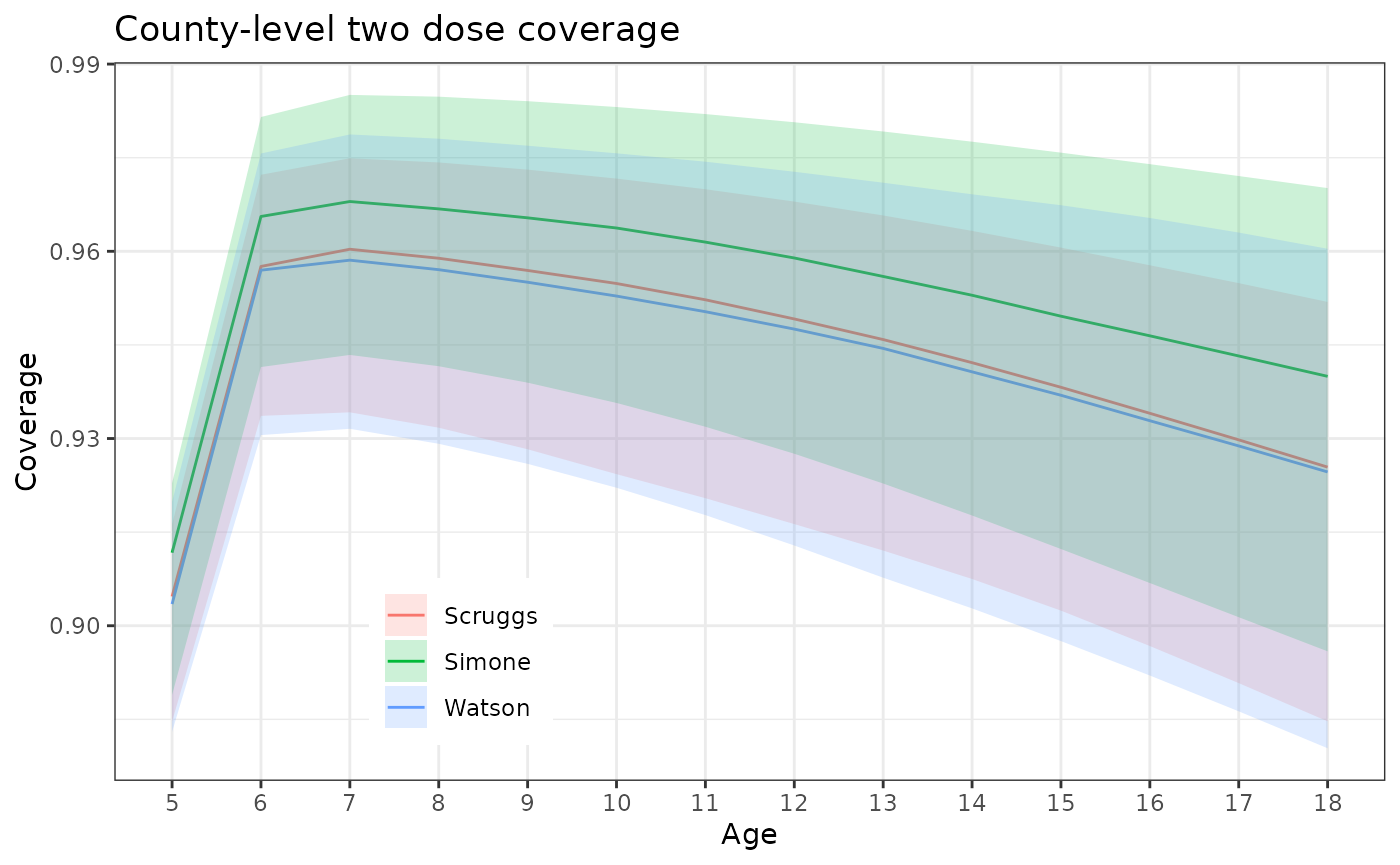
We can also look at the trend in coverage by age at the county level. Note that they follow the same trend as the state but with differing magnitude.
summary_predict |>
  subset(loc_id %in% c("Scruggs", "Simone", "Watson") & dose == 2 & age > 4) |>
  ggplot() +
  aes(x = age) +
  geom_line(aes(y = q50, color = loc_id)) +
  geom_ribbon(aes(ymin = q2_5, ymax = q97_5, fill = loc_id), alpha = 0.2) +
  theme_bw() +
  theme(
    legend.position = "inside", legend.position.inside = c(.2, 0.05),
    legend.justification.inside = c(0, 0)
  ) +
  scale_x_continuous(breaks = 5:18, minor_breaks = NULL) +
  scale_color_discrete(NULL, aesthetics = c("color", "fill")) +
  labs(
    x = "Age", y = "Coverage", title = "County-level two dose coverage"
  )
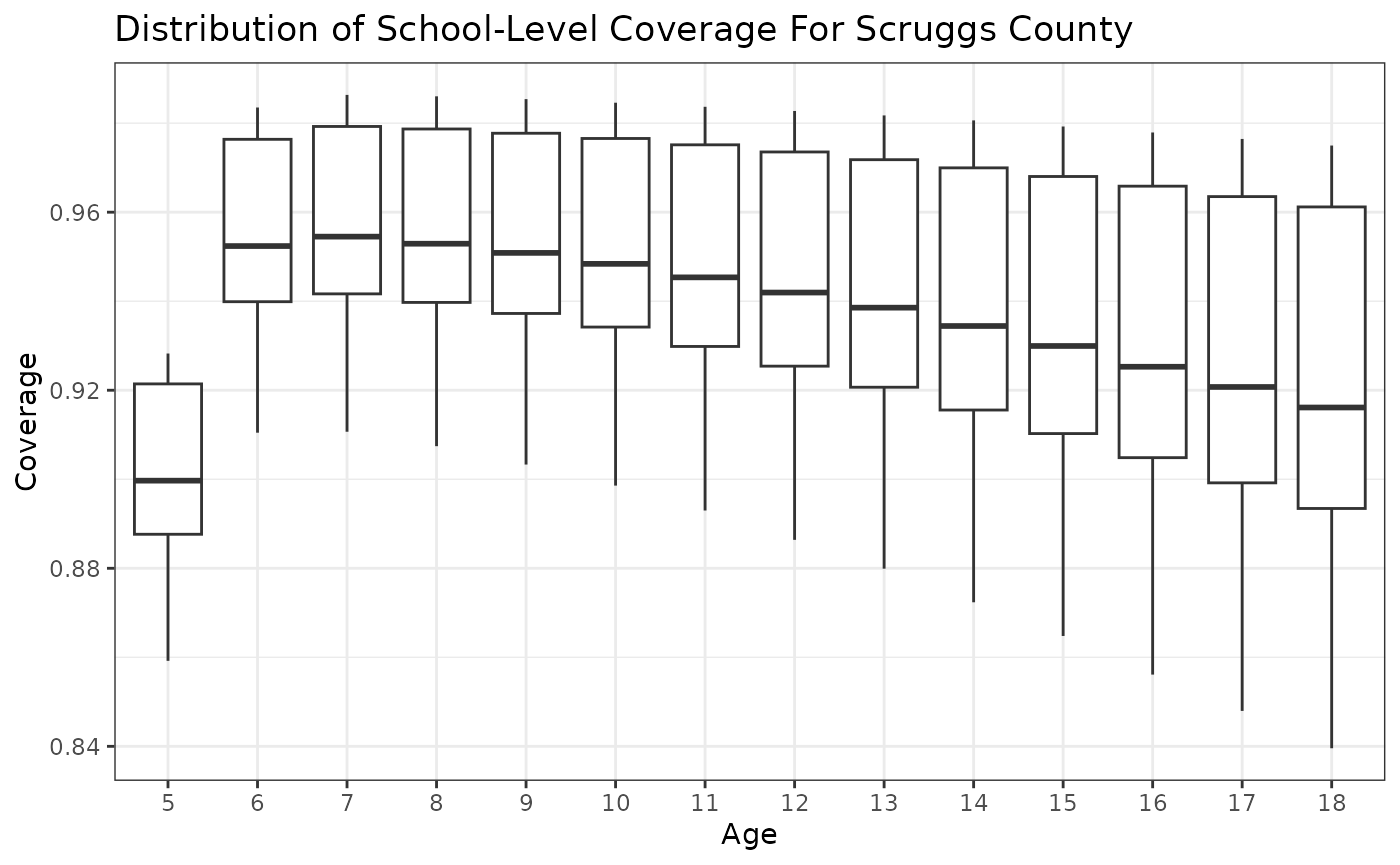
Next, we can look at the distribution of school-level coverage estimates by age group. Let’s focus on Scruggs County as an example.
scruggs_schools <- locations_sim[parent_id == "Scruggs", loc_id]
summary_predict |>
  subset(
    loc_id %in% scruggs_schools & dose == 2 & age > 4
  ) |>
  ggplot() +
  geom_boxplot(aes(x = factor(age), y = q50)) +
  theme_bw() +
  labs(
    x = "Age", y = "Coverage",
    title = "Distribution of School-Level Coverage For Scruggs County"
  )
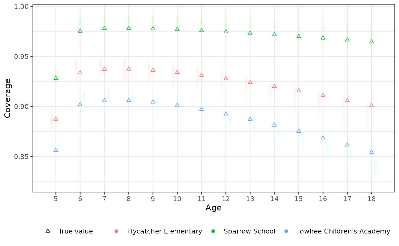
Finally let’s look at some selected schools and see how their predicted coverage compared to true underlying coverage from the data simulation process.
schools <- c(
  "Towhee Children's Academy", # ~380 per grade
  "Flycatcher Elementary", # ~110 per grade
  "Sparrow School" # ~60 per grade
)

# Subset to targets of interest (all retained posterior draws)
predict_sub <- predict_sim |>
  subset(loc_id %in% schools & dose == 2 & age > 4)

# Get the pre-computed background coverage matching the subsetted target
latent_ref <- copy(predict_sub$target)
latent_ref$coverage <- latent_params_sim$coverage[predict_sub$target$obs_id]


# Convert predictions to a long-format data.frame
draws_df <- as.data.frame(predict_sub)

# Now plot it all
ggplot() +
  aes(age, coverage, color = loc_id) +
  geom_point(
    data = draws_df,
    alpha = 1 / 256, shape = 16,
    position = position_jitterdodge(
      dodge.width = 0.5,
      jitter.width = 0.15
    )
  ) +
  geom_point(
    data = latent_ref,
    mapping = aes(shape = "True value"),
    fill = NA
  ) +
  theme_bw() +
  scale_shape_manual(
    name = "",
    values = c("True value" = 24)
  ) +
  scale_color_discrete(NULL, aesthetics = c("color", "fill")) +
  scale_x_continuous(breaks = 5:18, minor_breaks = NULL) +
  theme(legend.position = "bottom") +
  labs(color = "School", x = "Age", y = "Coverage")