Model Evaluation & PSIS-LOO Cross-Validation

Introduction

When evaluating model fit, you can use leave-one-out cross-validation (LOO-CV) to estimate out-of-sample predictive performance and identify highly influential observations without having to refit the MCMC model for every observation.

imuGAP provides S3 methods for rstantools::log_lik() and loo::loo(), enabling integration with the {loo} package (Vehtari et al. 2017, 2024) to compute Pareto Smoothed Importance Sampling Leave-One-Out (PSIS-LOO) diagnostics.

---

Computing the Pointwise Log-Likelihood

The rstantools::log_lik() method extracts the pointwise log-likelihood matrix for all $N$ observations across the $S$ posterior draws. For uncensored observations, it computes the binomial log probability mass; for left- or right-censored observations, it computes the corresponding cumulative log probability:

data("fit_sim", package = "imuGAP")
data("observations_sim", package = "imuGAP")
data("locations_sim", package = "imuGAP")

# Compute log-likelihood matrix (Draws x Observations)
ll_mat <- rstantools::log_lik(fit_sim)
#> 
#>  Elapsed Time: 0.289 seconds (Generated Quantities)
dim(ll_mat)
#> [1] 2000  841

---

Running PSIS-LOO and Inspecting Diagnostics

You can compute the Expected Log Pointwise Predictive Density ($\text{elpd}_{\text{loo}}$) and Pareto shape parameter $\hat{k}$ diagnostics by calling loo() directly on an imugap_fit object:

loo_res <- loo(fit_sim)
#> 
#>  Elapsed Time: 0.288 seconds (Generated Quantities)
print(loo_res)
#> 
#> Computed from 2000 by 841 log-likelihood matrix.
#> 
#>          Estimate   SE
#> elpd_loo  -2102.9 32.1
#> p_loo        26.2  1.5
#> looic      4205.7 64.3
#> ------
#> MCSE of elpd_loo is 0.7.
#> MCSE and ESS estimates assume MCMC draws (r_eff in [0.0, 0.9]).
#> 
#> All Pareto k estimates are good (k < 0.7).
#> See help('pareto-k-diagnostic') for details.

The Pareto shape parameter $\hat{k}$ diagnostic indicates whether importance weights have finite variance and gauges the reliability of the PSIS approximation (Vehtari et al. 2017, 2024):

• $\hat{k} < 0.5$ (including $< 0$): High reliability; importance weights have finite variance, and the central limit theorem holds.
• $0.5 \le \hat{k} < 0.7$: Moderate reliability; variance is finite, but convergence is slower.
• $\hat{k} \ge 0.7$: Influential observation; raw importance weights have high or infinite variance, meaning importance sampling estimates may be unreliable without exact refitting or moment matching.

In practice, if all observations have $\hat{k} < 0.7$, PSIS-LOO provides a fast and reliable leave-one-out cross-validation approximation without refitting.

---

Visualizing Pareto $\hat{k}$ Diagnostics

You can visualize the $\hat{k}$ diagnostics across all observations to check whether any specific surveillance streams or data sources exhibit high influence:

Show plot code

# Map observations to surveillance stream / layer type
loc_map <- canonicalize_locations(locations_sim)[, .(loc_id, layer)]
obs_meta <- canonicalize_observations(observations_sim, drop_extra = FALSE)
obs_meta <- merge(obs_meta, loc_map, by = "loc_id")
data.table::setorder(obs_meta, obs_c_id)

obs_meta[, stream := data.table::fcase(
  layer == 1L, "State Surveys",
  layer == 2L, "County Surveys (Censored)",
  layer == 3L, "School Entry"
)]

k_df <- data.frame(
  obs_idx = seq_along(loo_res$diagnostics$pareto_k),
  pareto_k = loo_res$diagnostics$pareto_k,
  stream = factor(obs_meta$stream, levels = c(
    "School Entry",
    "State Surveys",
    "County Surveys (Censored)"
  ))
)

ggplot(k_df, aes(x = obs_idx, y = pareto_k, color = stream)) +
  # Painted background regions for k thresholds
  annotate(
    "rect",
    xmin = -Inf,
    xmax = Inf,
    ymin = -Inf,
    ymax = 0.5,
    fill = "#2ca02c",
    alpha = 0.07
  ) +
  annotate(
    "rect",
    xmin = -Inf,
    xmax = Inf,
    ymin = 0.5,
    ymax = 0.7,
    fill = "#e6ab02",
    alpha = 0.12
  ) +
  annotate(
    "rect",
    xmin = -Inf,
    xmax = Inf,
    ymin = 0.7,
    ymax = Inf,
    fill = "#d95f02",
    alpha = 0.15
  ) +
  # Pareto k quantitative region labels
  annotate(
    "label",
    x = 10L,
    y = 0.75,
    label = "Influential (k >= 0.7)",
    hjust = 0,
    size = 3.2,
    fontface = "italic",
    color = "#b30000",
    fill = ggplot2::alpha("white", 0.6)
  ) +
  annotate(
    "label",
    x = 10L,
    y = 0.60,
    label = "Moderate (0.5 <= k < 0.7)",
    hjust = 0,
    size = 3.2,
    fontface = "italic",
    color = "#b37400",
    fill = ggplot2::alpha("white", 0.6)
  ) +
  annotate(
    "label",
    x = 10L,
    y = 0.40,
    label = "Reliable (k < 0.5)",
    hjust = 0,
    size = 3.2,
    fontface = "italic",
    color = "#006600",
    fill = ggplot2::alpha("white", 0.6)
  ) +
  geom_hline(yintercept = c(0.5, 0.7), linetype = "dashed", color = "grey40") +
  geom_point(alpha = 0.8, size = 2) +
  coord_cartesian(ylim = c(min(k_df$pareto_k, 0) - 0.05, max(k_df$pareto_k, 0.8) + 0.05)) +
  scale_color_brewer(palette = "Set2") +
  labs(
    title = "PSIS-LOO Pareto k Diagnostics",
    subtitle = "Observation influence diagnostic by surveillance stream",
    x = "Observation Index (Canonical ID)",
    y = "Pareto Shape Parameter (k)",
    color = "Surveillance Stream"
  ) +
  theme(legend.position = "bottom")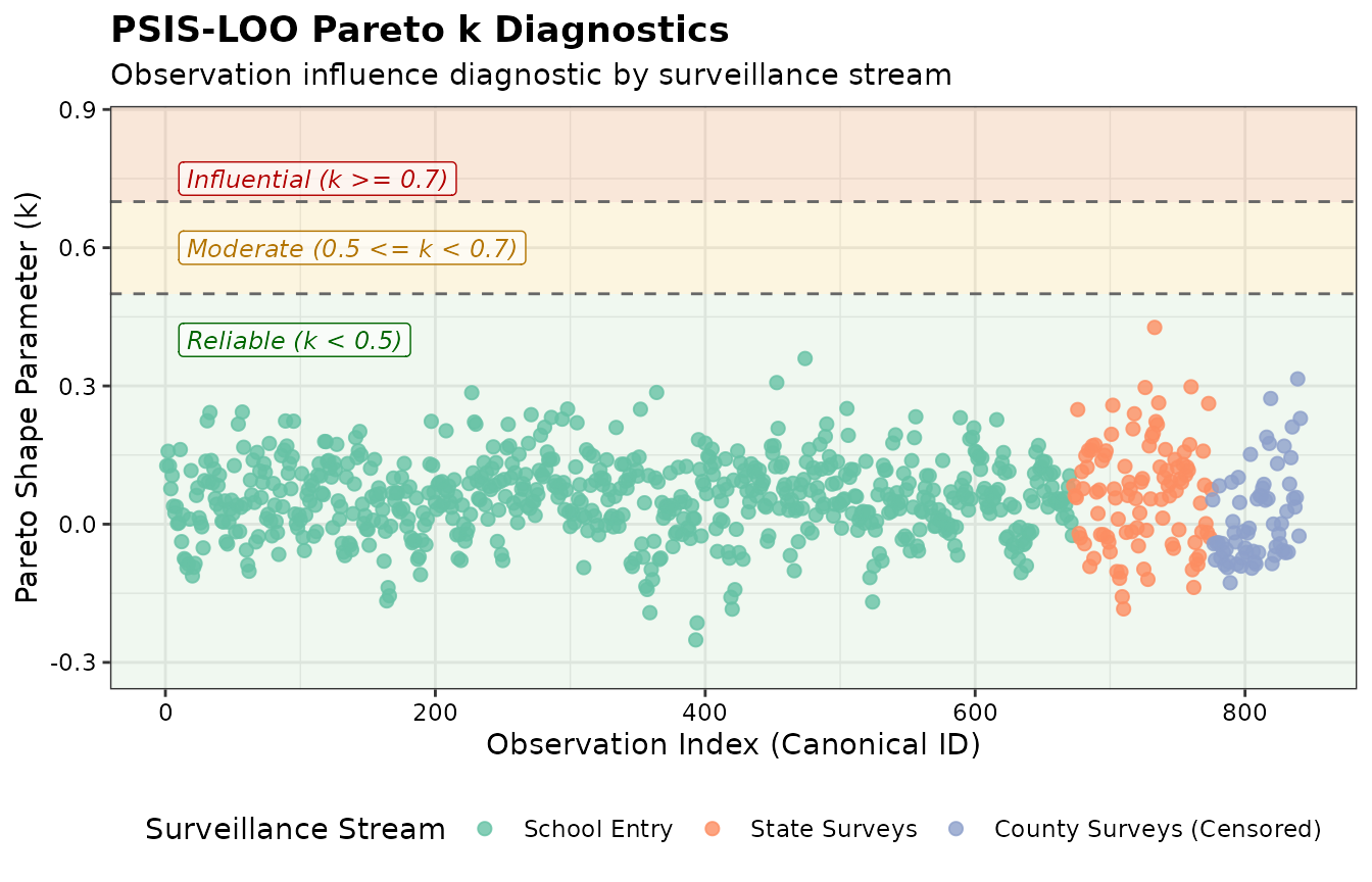

Pareto k influence diagnostics across surveillance streams

---

References

Vehtari, Aki, Andrew Gelman, and Jonah Gabry. 2017. “Practical Bayesian Model Evaluation Using Leave-One-Out Cross-Validation and WAIC.” Statistics and Computing 27 (5): 1413–32. https://doi.org/10.1007/s11222-016-9696-4.

Vehtari, Aki, Daniel Simpson, Andrew Gelman, Yuling Yao, and Jonah Gabry. 2024. “Pareto Smoothed Importance Sampling.” Journal of Machine Learning Research 25 (72): 1–58. https://jmlr.org/papers/v25/19-556.html.