4. Ensembling, Visualization, and Scoring Forecasting Outputs
Source:vignettes/04-utilizing-hub-output.Rmd
04-utilizing-hub-output.Rmd2) Get FluSight data repo
The FluSight Github repository stores forecast data for the FluSight Influenza Forecasting Hub, run by the US CDC. This project collects forecasts for weekly new hospitalizations due to confirmed influenza. More information can be found in the ReadMe of the repository: https://github.com/cdcepi/FluSight-forecast-hub.
We will copy a set of forecasts from this repository, and use them to build a simple ensemble, visualize the forecasts, and score them against observed data.
To switch to a different forecasting hub, change the
disease argument in the clone_hub_repos()
function below.
repo_dir <- clone_hub_repos(disease = forecast_disease,
                            clone_dir = getwd())
## Cloning repository...## Cloning into 'FluSight-forecast-hub'...
## Updating files: 36% (1004/2714)Updating files: 37% (1005/2714)Updating files: 38% (1032/2714)Updating files: 39% (1059/2714)Updating files: 40% (1086/2714)Updating files: 41% (1113/2714)Updating files: 42% (1140/2714)Updating files: 43% (1168/2714)Updating files: 44% (1195/2714)Updating files: 45% (1222/2714)Updating files: 46% (1249/2714)Updating files: 47% (1276/2714)Updating files: 48% (1303/2714)Updating files: 49% (1330/2714)Updating files: 50% (1357/2714)Updating files: 51% (1385/2714)Updating files: 52% (1412/2714)Updating files: 53% (1439/2714)Updating files: 54% (1466/2714)Updating files: 55% (1493/2714)Updating files: 56% (1520/2714)Updating files: 57% (1547/2714)Updating files: 58% (1575/2714)Updating files: 59% (1602/2714)Updating files: 60% (1629/2714)Updating files: 61% (1656/2714)Updating files: 62% (1683/2714)Updating files: 63% (1710/2714)Updating files: 64% (1737/2714)Updating files: 65% (1765/2714)Updating files: 66% (1792/2714)Updating files: 67% (1819/2714)Updating files: 68% (1846/2714)Updating files: 69% (1873/2714)Updating files: 69% (1897/2714)Updating files: 70% (1900/2714)Updating files: 71% (1927/2714)Updating files: 72% (1955/2714)Updating files: 73% (1982/2714)Updating files: 74% (2009/2714)Updating files: 75% (2036/2714)Updating files: 76% (2063/2714)Updating files: 77% (2090/2714)Updating files: 78% (2117/2714)Updating files: 79% (2145/2714)Updating files: 80% (2172/2714)Updating files: 81% (2199/2714)Updating files: 82% (2226/2714)Updating files: 83% (2253/2714)Updating files: 84% (2280/2714)Updating files: 85% (2307/2714)Updating files: 86% (2335/2714)Updating files: 87% (2362/2714)Updating files: 88% (2389/2714)Updating files: 89% (2416/2714)Updating files: 90% (2443/2714)Updating files: 91% (2470/2714)Updating files: 92% (2497/2714)Updating files: 93% (2525/2714)Updating files: 94% (2552/2714)Updating files: 95% (2579/2714)Updating files: 96% (2606/2714)Updating files: 97% (2633/2714)Updating files: 98% (2660/2714)Updating files: 98% (2672/2714)Updating files: 99% (2687/2714)Updating files: 100% (2714/2714)Updating files: 100% (2714/2714), done.## Using repo_dir: /home/runner/work/AMPH_Forecast_Suite/AMPH_Forecast_Suite/vignettes/FluSight-forecast-hubCopy specific forecast round to the model-output folder
We will copy forecasts from a set of models from FluSight. These include: # - FluSight-baseline # - MOBS-GLEAM_FLUH # - FluSight-ensemble
# models from flusight
models_to_copy <- c(
  "FluSight-baseline",
  "MOBS-GLEAM_FLUH",
  "FluSight-ensemble")

#models from AMPH
models_created_in_AMPH <- list.dirs("model-output",
                                    full.names = FALSE,
                                    recursive = FALSE)
# copy Forecast Hub forecasts to model-output folder
copy_fch_outputs(repo_dir,
                 reference_date,
                 models_to_copy)
## Copied files for date 2024-12-07 to /home/runner/work/AMPH_Forecast_Suite/AMPH_Forecast_Suite/vignettes/model-output4) Load model output (hub forecasts & your forecasts)
output_path <- file.path("model-output")

# Retrieve parquet/csv model output files and keep those matching the reference date
file_paths <- list.files(output_path, pattern = "\\.(parquet|csv)$",
                         full.names = TRUE, recursive = TRUE)
file_paths <- file_paths[grepl(reference_date, file_paths)]

if (!length(file_paths)) {
  stop("No model-output files found for reference_date = ", reference_date,
       ". Try a different date.")
}


# Read & bind; keep quantile forecasts; add model_id from folder name

projection_data_all <- file_paths %>%
  purrr::map_dfr(function(.x) {
    df <- read_model_file(.x)

    # standardize expected columns just in case
    if (!"output_type" %in% names(df))   stop("Missing 'output_type' in: ", .x)
    if (!"output_type_id" %in% names(df)) stop("Missing 'output_type_id' in: ", .x)

    df %>%
      dplyr::filter(.data$output_type == "quantile") %>%
      dplyr::mutate(
        output_type_id = suppressWarnings(as.numeric(.data$output_type_id)),
        model_id = basename(dirname(.x)),
        location = as.character(location)
      )
  })

prep_proj_data <- projection_data_all %>%
  dplyr::mutate(
    target_end_date = dplyr::coalesce(target_end_date, reference_date + 7 * as.integer(horizon))
  ) %>%
  dplyr::select(-tidyselect::any_of(c("model", "origin_date")))

# Convert to hubverse model_out_tbl format
projection_data_tbl <- hubUtils::as_model_out_tbl(prep_proj_data) %>%
  dplyr::filter(model_id %in% c(
    models_created_in_AMPH,
    models_to_copy
  ))


# Read and join location metadata (for names/abbreviations)

# loc_data <- readr::read_csv(file.path(dir_path, "auxiliary-data", "locations.csv"),
#                             show_col_types = FALSE)
data(loc_data, package = "AMPHForecastSuite")

projection_data_tbl2 <- projection_data_tbl %>%
  dplyr::left_join(
    loc_data %>%
        mutate(location = tolower(abbreviation)) %>%
            dplyr::select(location, location_name) %>%
      bind_rows(
        loc_data %>%
          dplyr::select(location, location_name)),
    by = "location"
  ) %>%
  dplyr::mutate(location_name = dplyr::coalesce(location_name, location))

dplyr::distinct(projection_data_tbl, model_id) %>% knitr::kable()| model_id |
|---|
| AMPH-epipredict-arx |
| AMPH-epipredict-climate |
| AMPH-neuralnetwork |
| AMPH-sarima |
| FluSight-baseline |
| FluSight-ensemble |
| MOBS-GLEAM_FLUH |
6) Build a simple equal-weight ensemble
We will use the simple_ensemble() function from the
hubEnsembles package to build a simple, equal-weight
ensemble across a set of models. In this example, we exclude the
FluSight-baseline and FluSight-ensemble, and only ensemble for a single
location and forecast date.
# Filter to the location of interest and the chosen forecast round
round_dat <- projection_data_tbl2 %>%
  dplyr::filter(.data$location_name == loc,
                target == target,
                output_type == "quantile",
                horizon >= 0) %>%
  dplyr::collect()

# Generate a simple (equal-weight) ensemble across contributing models
round_ens <- hubEnsembles::simple_ensemble(
  round_dat %>%
    dplyr::filter(model_id %in% c("AMPH-SARIMA","AMPH-neuralnetwork", "MOBS-GLEAM_FLUH"))) %>%
    # dplyr::filter(!(model_id %in% c("FluSight-baseline", "AMPH-SARIMA","AMPH-neuralnetwork",
    #                                 "FluSight-ensemble",
    #                                 "AMPH-epipredict-climate")))) %>%
  mutate(model_id = "AMPH-ensemble")

# Combine ensemble with individual models for plotting
plot_df <- dplyr::bind_rows(round_dat, round_ens)

# lapply(unique(round_dat$model_id), function(x){round_dat %>% filter(model_id==x) %>% pull(output_type_id) %>% unique() %>% length()})

unique(plot_df$model_id)
## [1] "AMPH-epipredict-arx" "AMPH-epipredict-climate"
## [3] "AMPH-neuralnetwork" "AMPH-sarima"
## [5] "FluSight-baseline" "FluSight-ensemble"
## [7] "MOBS-GLEAM_FLUH" "AMPH-ensemble"7) Prepare data for visualization
# pull updated target data
new_target_data_date <- lubridate::as_date(reference_date) + lubridate::weeks(5)
target_data_plot <- get_nhsn_data(
  disease = forecast_disease,
  geo_values = geo_ids,
  forecast_date = new_target_data_date,
  save_data = TRUE
)
## Important: forecast_date is more than 1 week ago. Pulling data issued prior to forecast_date.## Pulling data issued on or before 2025-01-11## Warning: No API key found. You will be limited to non-complex queries and encounter rate
## limits if you proceed.
## ℹ See `?save_api_key()` for details on obtaining and setting API keys.
## This warning is displayed once every 8 hours.
target_data_plot <- readr::read_csv(
  file.path("target-data", paste0("target-hospital-admissions-", new_target_data_date, ".csv")),
  show_col_types = FALSE)

# Forecasts to tidy plot
proj_data <- hubUtils::as_model_out_tbl(plot_df) %>%
  dplyr::rename(target_date = target_end_date) %>%
  dplyr::mutate(output_type_id = suppressWarnings(as.numeric(output_type_id))) %>%
  dplyr::arrange(model_id, horizon, target_date, output_type_id) %>%
  dplyr::distinct(model_id, horizon, target_date, output_type_id, .keep_all = TRUE)

# Observed data for the same location and time window
target_data_plot <- target_data_plot %>%
  dplyr::filter(target_end_date > start_date) %>%
  dplyr::rename(date = target_end_date)

head(proj_data)
## # A tibble: 6 × 10
## model_id target_date reference_date target horizon location location_name
## <chr> <date> <date> <chr> <dbl> <chr> <chr>
## 1 AMPH-ensemble 2024-12-07 2024-12-07 wk in… 0 24 Maryland
## 2 AMPH-ensemble 2024-12-07 2024-12-07 wk in… 0 24 Maryland
## 3 AMPH-ensemble 2024-12-07 2024-12-07 wk in… 0 24 Maryland
## 4 AMPH-ensemble 2024-12-07 2024-12-07 wk in… 0 24 Maryland
## 5 AMPH-ensemble 2024-12-07 2024-12-07 wk in… 0 24 Maryland
## 6 AMPH-ensemble 2024-12-07 2024-12-07 wk in… 0 24 Maryland
## # ℹ 3 more variables: output_type <chr>, output_type_id <dbl>, value <dbl>
head(target_data_plot)## # A tibble: 6 × 10
## location abbreviation location_name target source disease signal date
## <dbl> <chr> <chr> <chr> <chr> <chr> <chr> <date>
## 1 24 MD Maryland wk inc i… nhsn influe… confi… 2024-09-21
## 2 24 MD Maryland wk inc i… nhsn influe… confi… 2024-09-28
## 3 24 MD Maryland wk inc i… nhsn influe… confi… 2024-10-05
## 4 24 MD Maryland wk inc i… nhsn influe… confi… 2024-10-12
## 5 24 MD Maryland wk inc i… nhsn influe… confi… 2024-10-19
## 6 24 MD Maryland wk inc i… nhsn influe… confi… 2024-10-26
## # ℹ 2 more variables: issue_date <date>, observation <dbl>8) Plot forecasts vs. truth
We use two different approaches to visualize the forecasts
vs. observed data. The hubVis package provides a convenient
function to plot forecasts,
plot_step_ahead_model_output().
We can also plot ggplot2 directly, though this requires
more code.
Option 1: with hubVis
# This is having issues

hubVis::plot_step_ahead_model_output(
  proj_data,
  target_data = target_data_plot,
  use_median_as_point = TRUE,
  show_legend = TRUE,
  intervals = 0.8,
  ens_name = "AMPH-ensemble",
  ens_color = "black"
)
Option 2: with ggplot2
library(dplyr)
library(tidyr)
library(ggplot2)
library(scales)

# target_data_plot <- readr::read_csv(
#   file.path("target-data", paste0("target-hospital-admissions-", new_target_data_date, ".csv")),
#   show_col_types = FALSE)

# Identify ensemble id from the object you created earlier
ens_id <- unique(round_ens$model_id)[1]  # e.g., "hub-ensemble"

# Build the 80% ribbon (0.1 / 0.9) for all models
ribbon_80 <- proj_data %>%
  filter(output_type == "quantile", output_type_id %in% c(0.1, 0.9)) %>%
  mutate(output_type_id = as.numeric(output_type_id)) %>%
  select(model_id, horizon, target_date, output_type_id, value) %>%
  pivot_wider(names_from = output_type_id, values_from = value, names_prefix = "q") %>%
  rename(ymin = q0.1, ymax = q0.9)

# Median (0.5) for all models
med_50 <- proj_data %>%
  filter(output_type == "quantile", output_type_id == 0.5) %>%
  select(model_id, horizon, target_date, value) %>%
  mutate(line_width = if_else(model_id == ens_id, 1.1, 0.8))

# Legend order: others first, ensemble last
model_levels <- proj_data %>%
  distinct(model_id) %>%
  pull(model_id) %>%
  setdiff(ens_id) %>%
  c(ens_id)

# Okabe–Ito palette (color-blind friendly)
okabe_ito <- c(
  "#E69F00", "#56B4E9", "#009E73", "#F0E442",
  "#0072B2", "#D55E00", "#CC79A7", "#999999"
)
n_other <- length(model_levels) - 1

other_cols <- if (n_other <= length(okabe_ito)) okabe_ito[seq_len(n_other)] else scales::hue_pal(l = 45, c = 100)(n_other)

# Lines: others = Okabe–Ito, ensemble = black
color_vals <- setNames(c(other_cols, "#000000"), model_levels)
# Ribbons: same hues; ensemble darker gray so black line pops
fill_vals  <- setNames(c(other_cols, "#3A3A3A"), model_levels)

ggplot() +
  geom_ribbon(
    data = ribbon_80,
    aes(x = target_date, ymin = ymin, ymax = ymax, fill = model_id),
    alpha = 0.22, show.legend = TRUE
  ) +
  geom_line(
    data = med_50,
    aes(x = target_date, y = value, color = model_id, linewidth = line_width),
    lineend = "round", alpha = 0.98, show.legend = TRUE
  ) +
  geom_point(
    data = target_data_plot,
    aes(x = date, y = observation),
    size = 1.2, alpha = 0.85, inherit.aes = FALSE,
    color = "grey50"
  ) +
  geom_line(
    data = target_data_plot,
    aes(x = date, y = observation),
    alpha = 0.85, inherit.aes = FALSE,
    color = "grey50"
  ) +
  scale_color_manual(values = color_vals, name = "Model") +
  scale_fill_manual(values  = fill_vals,  name = "Model") +
  scale_linewidth_identity() +
  labs(x = "Target date", y = "Weekly incident hospitalizations") +
  theme_minimal(base_size = 12) +
  theme(legend.position = "right")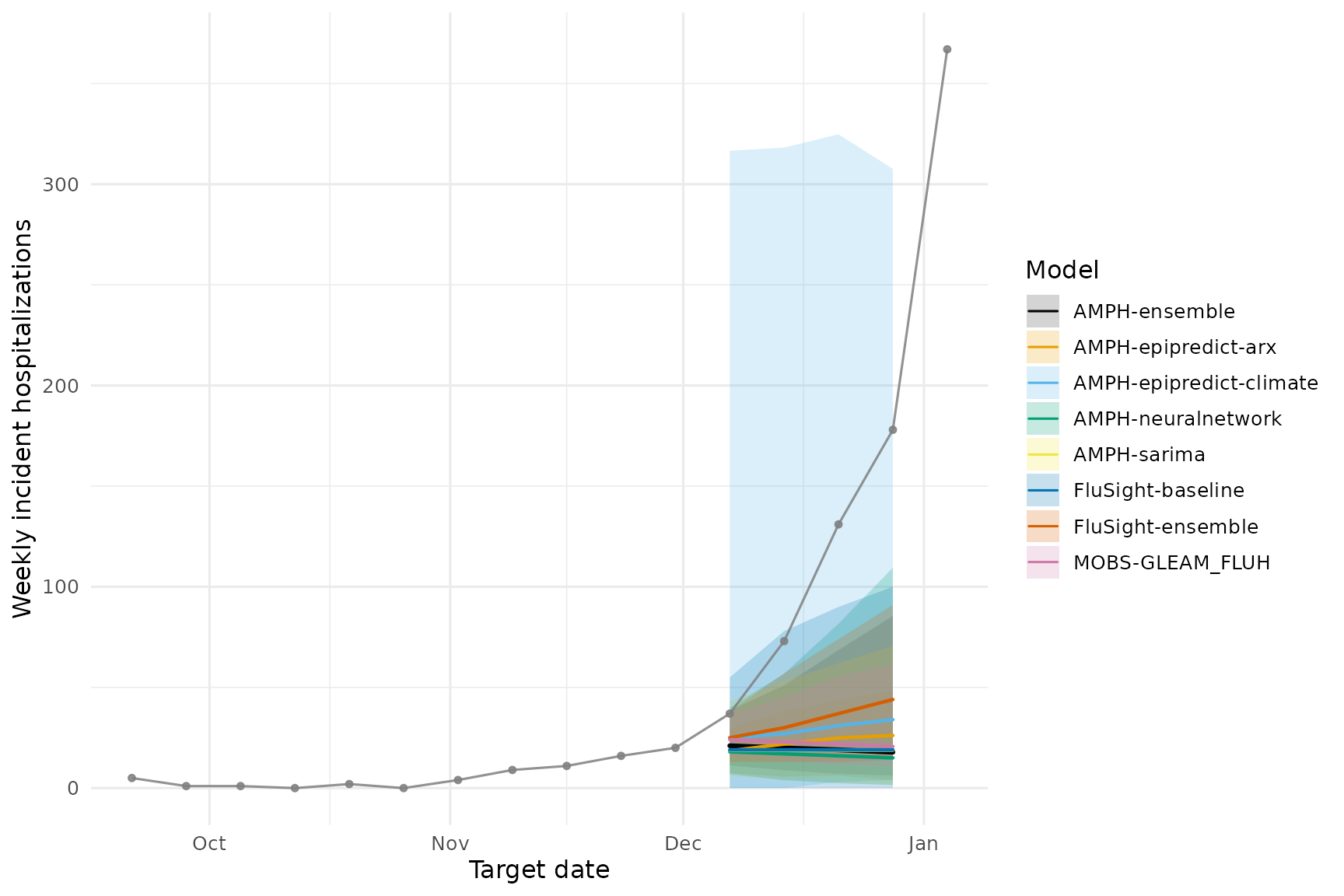
10) Score forecasts (WIS, coverage)
Evaluation of forecasts is critical for assessing model performance
and for building trust in forecasts. Proper scoring rules, such as the
Weighted Interval Score (WIS), provide a way to evaluate the accuracy
and calibration of probabilistic forecasts. Scoring requires observed
data. We will use the scoringutils package to compute WIS
for our forecasts.
scoring_target_data <- readr::read_csv(
  file.path("target-data", paste0("target-hospital-admissions-", new_target_data_date, ".csv")),
  show_col_types = FALSE)

scoring_target_data <- scoring_target_data %>%
  filter(location %in% location,
         issue_date >= target_end_date,
         target_end_date > "2022-09-01") %>%
  select(geo_value = location, target_end_date, value = observation) %>%
  drop_na(value) %>%
  epiprocess::as_epi_df(time_value = target_end_date)
# Join forecasts with observations at (target_date, location)
# and conform to scoringutils "forecast" structure.

scoring_df <- dplyr::left_join(
  proj_data,
  scoring_target_data %>%
    dplyr::rename(observation = value,
                  target_date = time_value) %>%
    mutate(location_name = loc) %>%
    select(-geo_value),
  by = c("target_date", "location_name"),
  relationship = "many-to-one"
) %>%
  dplyr::rename(
    model = model_id,
    predicted = value,
    observed = observation,
    quantile_level = output_type_id
  )

# Convert to a scoringutils forecast object
forecast <- scoringutils::as_forecast_quantile(
  scoring_df,
  observed       = "observed",
  predicted      = "predicted",
  quantile_level = "quantile_level",
  # be explicit so extra cols don't confuse the unit of a single forecast
  forecast_unit  = c("model", "location_name", "target_date")
)

# Score (WIS, coverage, etc.)
scores <- scoringutils::score(forecast)
knitr::kable(scoringutils::summarise_scores(scores, by = "model"))| model | wis | overprediction | underprediction | dispersion | bias | interval_coverage_50 | interval_coverage_90 | ae_median |
|---|---|---|---|---|---|---|---|---|
| AMPH-ensemble | 57.72073 | 0 | 53.93871 | 3.782014 | -0.9200 | 0 | 0.25 | 85.29844 |
| AMPH-epipredict-arx | 62.20304 | 0 | 58.88705 | 3.315985 | -0.9525 | 0 | 0.25 | 81.89191 |
| AMPH-epipredict-climate | 39.23780 | 0 | 11.72917 | 27.508632 | -0.3500 | 1 | 1.00 | 75.50000 |
| AMPH-neuralnetwork | 55.28833 | 0 | 50.30912 | 4.979213 | -0.9000 | 0 | 0.50 | 88.23638 |
| AMPH-sarima | 61.90821 | 0 | 57.58205 | 4.326163 | -0.9125 | 0 | 0.25 | 85.92319 |
| FluSight-baseline | 54.71011 | 0 | 48.66304 | 6.047065 | -0.8825 | 0 | 0.50 | 85.75000 |
| FluSight-ensemble | 50.65141 | 0 | 46.18478 | 4.466630 | -0.9325 | 0 | 0.25 | 70.75000 |
| MOBS-GLEAM_FLUH | 62.53968 | 0 | 59.95487 | 2.584814 | -0.9700 | 0 | 0.25 | 82.36050 |