3. Forecasting with Time Series Models

Setup

Set parameters

state_name <- "Maryland"
geo_ids <- "md"
forecast_date <- as.Date("2024-12-01")
forecast_disease <- "influenza"
target <- "wk inc flu hosp"
forecast_horizon_wks <- 0:3

Load packages

knitr::opts_chunk$set(echo = TRUE)

library(AMPHForecastSuite)
library(tidyverse)
library(forecast)
library(jsonlite)
library(epidatr)
library(epipredict)
library(epiprocess)
library(ggplot2)
library(dplyr)

Load target (observed) data

We already pulled and saved the data we need in Collect Empirical Data. See vignettes/collect_empirical_data.Rmd for details.

# Load data saved from a specific forecast date: 
target_data_path <- file.path("target-data", paste0("target-hospital-admissions-", forecast_date, ".csv"))

target_data <- readr::read_csv(file = target_data_path) %>%
  mutate(location = as.character(location)) %>%
  dplyr::filter(!is.na(observation)) %>%        # keep rows with observed values
  dplyr::arrange(dplyr::across(dplyr::any_of(c("target_end_date","date"))))



# get location id to add to forecast output
location_dat <- target_data %>%
  dplyr::select(location, abbreviation, location_name) %>%
  distinct() 
location <- as.character(location_dat$location)

Define Reference date

The reference_date is the Saturday for the week of the forecast date. This is the date that will be used in the forecast submission file.

reference_date <- get_reference_date(forecast_date)

## Reference date: 2024-12-07

## Forecast date: 2024-12-01

Models

SARIMA (`forecast` package)

Here we use the auto.arima function from the forecast package to fit a seasonal ARIMA model to the data (seasonal = T). Use (seasonal = F) to remove seasonality.

Set the name

model_name <- "AMPH-sarima"

Run the model

fc_sarima <- forecast::auto.arima(y = target_data$observation, 
                                  seasonal = T, 
                                  lambda = "auto") %>%
  forecast::forecast(h = length(forecast_horizon_wks),
           level = c(.1, .2, .3, .4, 0.5, 0.6, 0.7, 0.8, 0.9, 0.95, 0.98))

## Warning in guerrero(x, lower, upper): Guerrero's method for selecting a Box-Cox
## parameter (lambda) is given for strictly positive data.

Plot SARIMA forecast results

# Build data for plotting
h <- length(forecast_horizon_wks)

# dates for history + horizon (uses target_end_date if present; else index)
hist_dates <- if ("target_end_date" %in% names(target_data)) as.Date(target_data$target_end_date) else seq_len(nrow(target_data))
fc_dates   <- if (is.Date(hist_dates)) max(hist_dates) + 7L*seq_len(h) else max(hist_dates) + seq_len(h)

df_hist <- data.frame(date = hist_dates, value = target_data$observation)

pick <- function(mat, lvl){
  nm <- paste0(lvl, "%")
  if (!is.null(colnames(mat)) && nm %in% colnames(mat)) mat[, nm] else mat[, ncol(mat)]
}

df_fc <- data.frame(
  date = fc_dates,
  mean = as.numeric(fc_sarima$mean),
  l80  = as.numeric(pick(fc_sarima$lower, 80)),
  u80  = as.numeric(pick(fc_sarima$upper, 80)),
  l95  = as.numeric(pick(fc_sarima$lower, 95)),
  u95  = as.numeric(pick(fc_sarima$upper, 95))
)

# keep only the last 10 observed points to view most recent data
df_hist_last <- df_hist %>% arrange(date) %>% slice_tail(n = 10)

# x-range: last observed window through end of forecast
x_start <- min(df_hist_last$date)
x_end   <- max(df_fc$date)

ggplot() +
  geom_point(data = df_hist_last, aes(date, value)) +
  geom_ribbon(data = df_fc, aes(date, ymin = l95, ymax = u95), alpha = 0.15) +
  geom_ribbon(data = df_fc, aes(date, ymin = l80, ymax = u80), alpha = 0.25) +
  geom_line(data = df_fc, aes(date, mean)) +
  coord_cartesian(xlim = c(x_start, x_end)) +
  labs(title = "SARIMA model fit and forecast",
       x = "Date", y = "Hospital admissions") +
  theme_minimal(base_size = 12)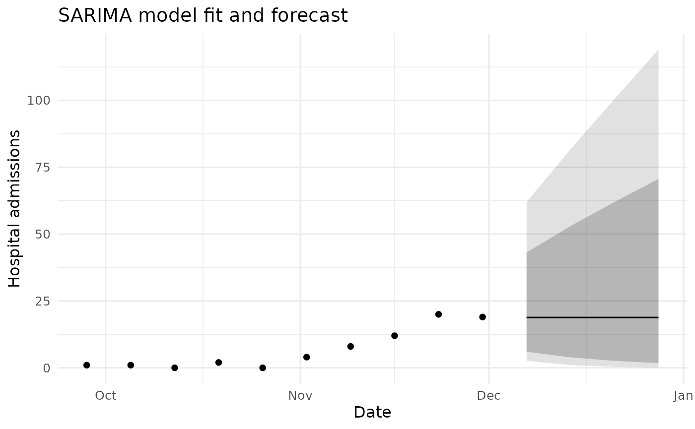

SARIMA model fit and forecast

Check that the model output is in the correct format.

We use the hubValidations package to check against the tasks.json file we create in Getting Started.

# Future functionality. Not yet developed.

Save in hubVerse Format

# Transform to hubVerse format
data_fc_sarima <- trans_forecastpkg_hv(fc_output = fc_sarima,
                                     model_name = model_name,
                                     target = target,
                                     reference_date = reference_date,
                                     horizon_time_steps = forecast_horizon_wks,
                                     geo_ids = location)


## Save data file
#' -- this will have validation build in for fluid workflow eventually.
save_model_output(model_name = model_name,
                  fc_output = data_fc_sarima,
                  reference_date)

## Model output saved to model-output/AMPH-sarima/2024-12-07-AMPH-sarima.csv

Neural network model (`forecast` package)

Here we use the nnetar function from the forecast package to fit a neural network model to the data.

Set the name

model_name <- "AMPH-neuralnetwork"

Run the model

fc_nnet <- forecast::nnetar(target_data$observation, 
                            lambda = "auto") %>%
  forecast(PI = TRUE,
           h = length(forecast_horizon_wks),
           level = c(.1, .2, .3, .4, 0.5, 0.6, 0.7, 0.8, 0.9, 0.95, 0.98))

## Warning in guerrero(x, lower, upper): Guerrero's method for selecting a Box-Cox
## parameter (lambda) is given for strictly positive data.

Plot Neural Network forecast results

df_fc <- data.frame(
  date = fc_dates,
  mean = as.numeric(fc_nnet$mean),
  l80  = as.numeric(pick(fc_nnet$lower, 80)),
  u80  = as.numeric(pick(fc_nnet$upper, 80)),
  l95  = as.numeric(pick(fc_nnet$lower, 95)),
  u95  = as.numeric(pick(fc_nnet$upper, 95))
)

ggplot() +
  geom_point(data = df_hist_last, aes(date, value)) +
  geom_ribbon(data = df_fc, aes(date, ymin = l95, ymax = u95), alpha = 0.15) +
  geom_ribbon(data = df_fc, aes(date, ymin = l80, ymax = u80), alpha = 0.25) +
  geom_line(data = df_fc, aes(date, mean)) +
  coord_cartesian(xlim = c(x_start, x_end)) +
  labs(title = "Neural network model fit and forecast",
       x = "Date", y = "Hospital admissions") +
  theme_minimal(base_size = 12)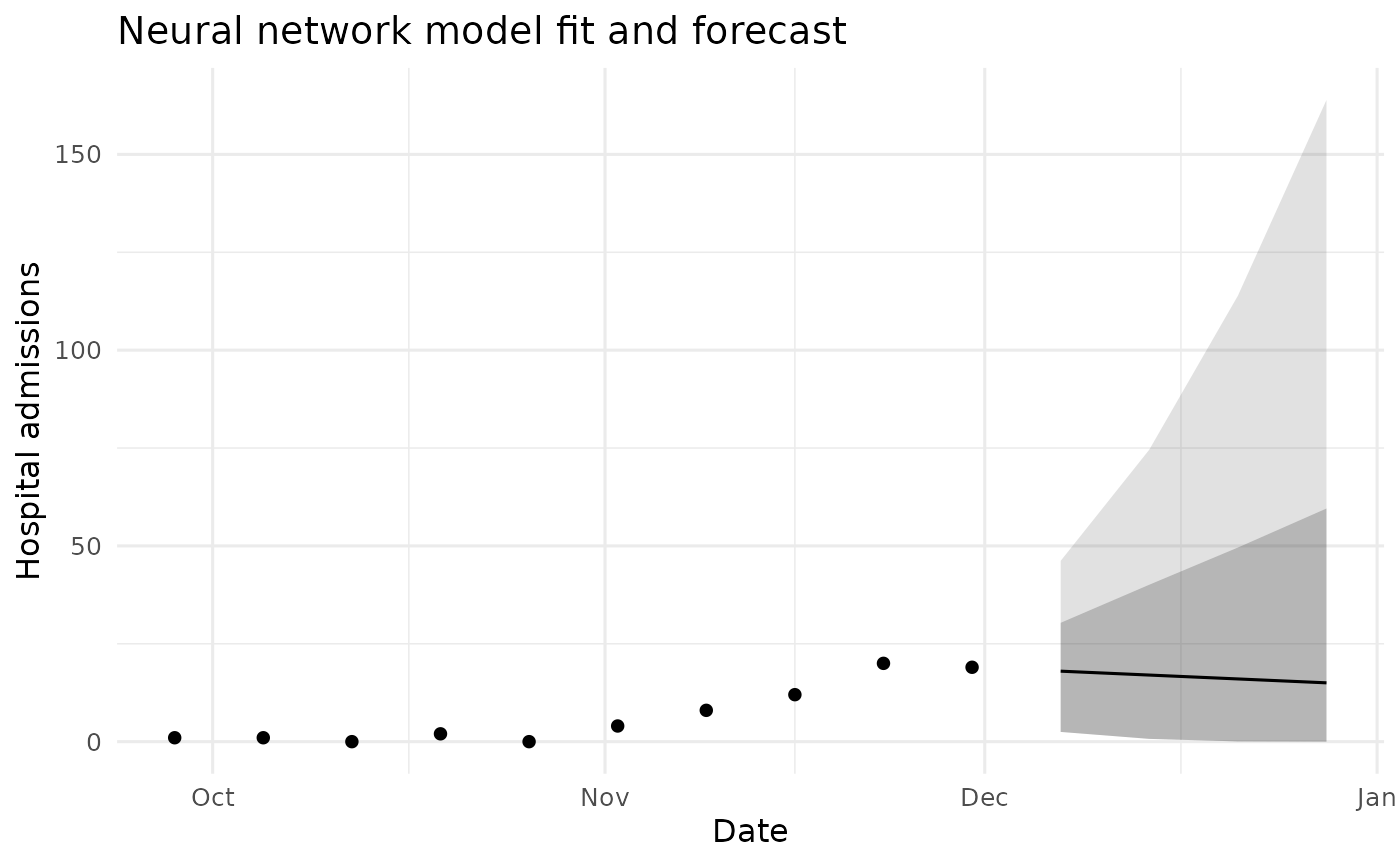

Neural network model fit and forecast

Save in hubVerse Format

# Transform to hubVerse format
data_fc_nnet <- trans_forecastpkg_hv(fc_output = fc_nnet,
                                     model_name = model_name,
                                     target = target,
                                     reference_date = reference_date,
                                     horizon_time_steps = forecast_horizon_wks,
                                     geo_ids = location)

## Save data file
#' -- this will have validation build in for fluid workflow eventually.
save_model_output(model_name = model_name,
                  fc_output = data_fc_nnet,
                  reference_date)

## Model output saved to model-output/AMPH-neuralnetwork/2024-12-07-AMPH-neuralnetwork.csv

Autoregressive Forecaster (`epipredict` package)

Here we use the epipredict package to fit an autoregressive model to the data. We specify lags of 0, 7, and 14 days (i.e., current week, previous week, and two weeks ago) and forecast horizons of 7, 14, 21, and 28 days ahead (i.e., 1 to 4 weeks ahead).

Set the name

model_name <- "AMPH-epipredict-arx"

Run the model

# Set up data for epipredict
target_data_arx <- target_data %>%
  rename(geo_value = location,
         time_value = target_end_date,
         value = observation) %>%
  tsibble::as_tsibble(index = time_value, key = c(geo_value)) %>%
  arrange(geo_value, time_value) %>%
  epiprocess::as_epi_df()

# Run model
arx_forecast <- lapply(
  seq(7, 28, 7),
  function(days_ahead) {
    epipredict::arx_forecaster(
      epi_data = target_data_arx, 
      outcome = "value",
      trainer = linear_reg(),
      predictors = "value",
      args_list = arx_args_list(
        lags = list(c(0, 7, 14)),
        ahead = days_ahead,
        quantile_levels = c(0.01, 0.025,
                            0.05, 0.1, 0.15, 0.2, 0.25, 0.3, 0.35,
                            0.4, 0.45, 0.5, 0.55, 0.6, 0.65, 0.7,
                            0.75, 0.8, 0.85, 0.9, 0.95,
                            0.975, 0.99),
        nonneg = TRUE
      )
    )
  }
)

# pull out the workflow and the predictions to be able to effectively use autoplot
arx_forecaster_workflow <- arx_forecast[[1]]$epi_workflow
arx_forecaster_results <- arx_forecast %>%
  purrr::map(~ `$`(., "predictions")) %>%
  list_rbind() %>%
  mutate(horizon = forecast_horizon_wks,
         location_id = state_name,
         model = model_name,
         target = target)
autoplot(
  object = arx_forecaster_workflow,
  predictions = arx_forecaster_results,
  observed_response = target_data_arx %>%
    filter(geo_value %in% geo_ids, time_value > (lubridate::as_date(forecast_date) - 4*30))) +
  geom_vline(aes(xintercept = forecast_date))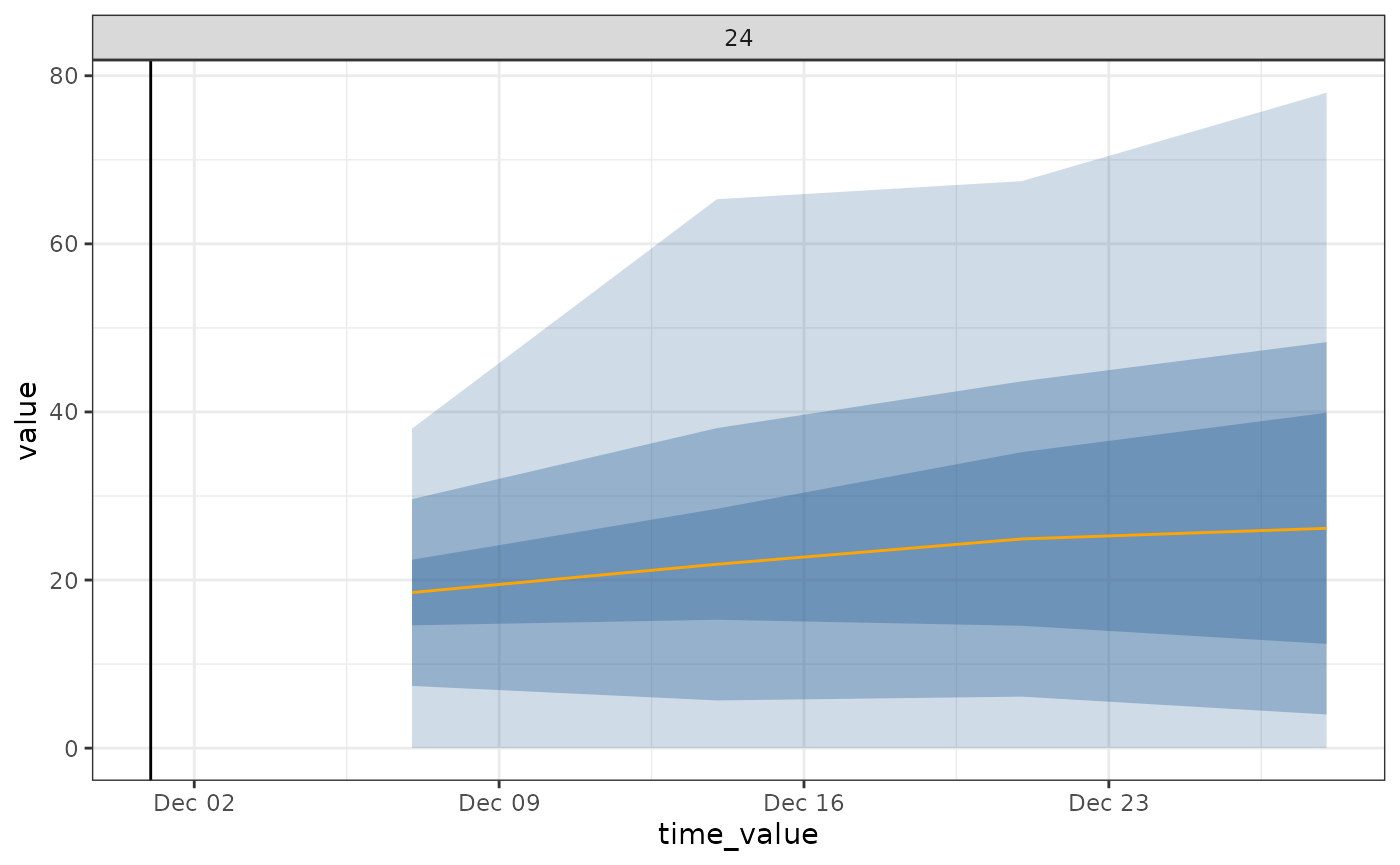

ARX model fit and forecast

Save in hubVerse Format

# Transform to hubVerse format
data_fc_arx_epipred <- trans_epipredarx_hv(fc_output = arx_forecast,
                                           model_name = model_name,
                                           target = target,
                                           reference_date = reference_date,
                                           horizon_time_steps = forecast_horizon_wks)

## Save data file
#' -- this will have validation build in for fluid workflow eventually.
save_model_output(model_name = model_name,
                  fc_output = data_fc_arx_epipred,
                  reference_date)

## Model output saved to model-output/AMPH-epipredict-arx/2024-12-07-AMPH-epipredict-arx.csv

Climatological Forecaster (`epipredict` package)

Here we use the epipredict package to fit a climatological model to the data. We specify a forecast horizon of 7, 14, 21, and 28 days ahead (i.e., 1 to 4 weeks ahead).

Set the name

model_name <- "AMPH-epipredict-climate"

Run the model

# Set up data for epipredict
target_data_clim <- target_data %>%
  rename(geo_value = location,
         time_value = target_end_date,
         value = observation) %>%
  tsibble::as_tsibble(index = time_value, key = c(geo_value)) %>%
  arrange(geo_value, time_value) %>%
  epiprocess::as_epi_df()

# Run the model
climate_forecast <- epipredict::climatological_forecaster(
  target_data_clim,
  outcome = "value",
  args_list = climate_args_list(
    forecast_horizon = forecast_horizon_wks,
    time_type = "week",
        quantile_levels = c(0.01, 0.025,
                            0.05, 0.1, 0.15, 0.2, 0.25, 0.3, 0.35,
                            0.4, 0.45, 0.5, 0.55, 0.6, 0.65, 0.7,
                            0.75, 0.8, 0.85, 0.9, 0.95,
                            0.975, 0.99),
    center_method = "median",
    quantile_by_key = "geo_value",
    forecast_date = reference_date,
    nonneg = TRUE
  )
)
climate_forecast_workflow <- climate_forecast$epi_workflow
climate_forecast_results <- climate_forecast$predictions %>%
  mutate(horizon = forecast_horizon_wks,
         location_id = state_name,
         model = model_name,
         target = target)

autoplot(
  object = climate_forecast_workflow,
  predictions = climate_forecast_results,
  observed_response = target_data_clim %>%
    filter(geo_value %in% geo_ids, time_value > (lubridate::as_date(forecast_date) - 4*30))) +
  geom_vline(aes(xintercept = forecast_date))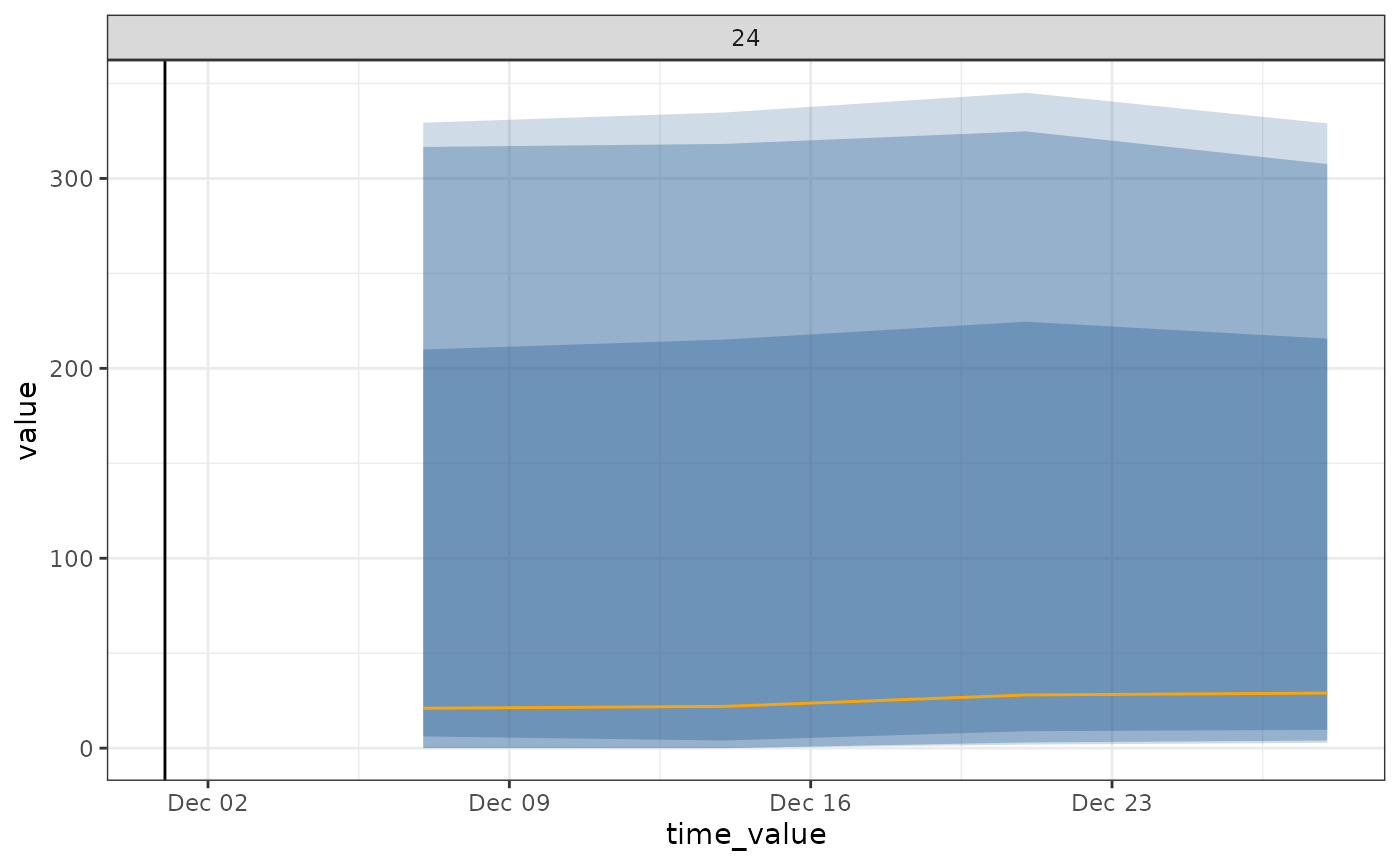

Climate model fit and forecast

Save in hubVerse Format

# Transform to hubVerse format
data_fc_climate_epipred <- trans_epipredclim_hv(fc_output = climate_forecast,
                                     model_name = model_name,
                                     target = target,
                                     reference_date = reference_date,
                                     horizon_time_steps = forecast_horizon_wks)

## Save data file
#' -- this will have validation build in for fluid workflow eventually.
save_model_output(model_name = model_name,
                  fc_output = data_fc_climate_epipred,
                  reference_date)

## Model output saved to model-output/AMPH-epipredict-climate/2024-12-07-AMPH-epipredict-climate.csv

Setup

Set parameters

Load packages

Load target (observed) data

Define Reference date

Models

SARIMA (forecast package)

Set the name

Run the model

Plot SARIMA forecast results

Check that the model output is in the correct format.

Save in hubVerse Format

Neural network model (forecast package)

Set the name

Run the model

Plot Neural Network forecast results

Save in hubVerse Format

Autoregressive Forecaster (epipredict package)

Set the name

Run the model

Save in hubVerse Format

Climatological Forecaster (epipredict package)

Set the name

Run the model

Save in hubVerse Format

SARIMA (`forecast` package)

Neural network model (`forecast` package)

Autoregressive Forecaster (`epipredict` package)

Climatological Forecaster (`epipredict` package)