Named-axis kernel products

Two different axes can index a rectangular parameter table. For example, K[consumer,resource] has one row for each consumer and one column for each resource. State arrays need not have the same length. The named selectors identify which axis is summed, including when the matrix is used in the opposite direction.

Expression	Independent array calculation
apply_along(K[consumer,resource:r]*P[resource:r], resource=r, kernel=sum)	K @ P
apply_along(g[consumer:c]*K[consumer:c,resource]*Z[consumer:c], consumer=c, kernel=sum)	K.T @ (g * Z)

The normalizer infers the parameter's axis order from its named references; validate_spec(spec).parameters reports the contract. Supply K with the reported shape and order. Distinct axis names make the intended row/column roles explicit, rather than relying on equal lengths to conceal a transpose.

The complete executable example includes both products and a per-coordinate choice of linear or quadratic loss:

"""Two distinct named axes, rectangular interactions and conditional losses.

Run ``uv run python examples/named_kernel_products.py``. All inputs are
synthetic. The independent reference uses ordinary matrix products.
"""

from __future__ import annotations

from typing import Any

import numpy as np

from op_system import compile_spec


def model_spec(resources: int = 3, consumers: int = 2) -> dict[str, Any]:
    """Describe interaction between two differently sized groups of variables.

    Returns:
        A specification with resource and consumer axes and a rectangular table.
    """
    return {
        "kind": "expr",
        "axes": [
            {"name": "resource", "coords": [f"r{i}" for i in range(resources)]},
            {"name": "consumer", "coords": [f"c{i}" for i in range(consumers)]},
        ],
        "state": ["P[resource]", "Z[consumer]"],
        "aliases": {
            "exposure[consumer]": (
                "apply_along(K[consumer,resource:r]*P[resource:r], "
                "resource=r, kernel=sum)"
            ),
            "removal[resource]": (
                "apply_along(g[consumer:c]*K[consumer:c,resource]*Z[consumer:c], "
                "consumer=c, kernel=sum)"
            ),
        },
        "equations": {
            "P[resource]": "-P[resource]*removal[resource]",
            "Z[consumer]": (
                "efficiency[consumer]*Z[consumer]*exposure[consumer] - "
                "np.where(linear[consumer] > 0, loss[consumer]*Z[consumer], "
                "loss[consumer]*Z[consumer]*Z[consumer])"
            ),
        },
    }


def inputs(resources: int = 3, consumers: int = 2) -> tuple[np.ndarray, dict[str, Any]]:
    """Return seeded states and a table ordered as consumer by resource."""
    rng = np.random.default_rng(312)
    state = rng.uniform(0.3, 2.0, size=resources + consumers)
    params = {
        "K": rng.uniform(0.0, 1.0, size=(consumers, resources)) / resources,
        "g": rng.uniform(0.2, 1.0, size=consumers),
        "efficiency": rng.uniform(0.2, 0.8, size=consumers),
        "loss": rng.uniform(0.05, 0.3, size=consumers),
        "linear": np.arange(consumers) % 2,
    }
    return state, params


def reference(state: np.ndarray, params: dict[str, Any]) -> np.ndarray:
    """Compute the same equations directly, without the specification compiler.

    Returns:
        Flat resource and consumer derivatives in declared state order.
    """
    consumers, resources = params["K"].shape
    p, z = state[:resources], state[resources : resources + consumers]
    resource_loss = -p * (params["K"].T @ (params["g"] * z))
    consumer_change = params["efficiency"] * z * (params["K"] @ p) - np.where(
        params["linear"] > 0, params["loss"] * z, params["loss"] * z**2
    )
    return np.concatenate([resource_loss, consumer_change])


def main() -> None:
    """Check the compiled equations against the independent rectangular product."""
    state, params = inputs()
    compiled = compile_spec(model_spec())
    result = compiled.eval_fn(0.0, state, **params)
    np.testing.assert_allclose(result, reference(state, params), rtol=1e-13, atol=1e-14)
    print(result)  # ruff: ignore[print] - command-line example output


if __name__ == "__main__":
    main()

Run uv run python examples/named_kernel_products.py. The example compares the compiled derivative with a separate NumPy implementation. Required backend qualification tests rectangular cases in NumPy, JAX and CPU PyTorch; JAX JIT and derivatives and PyTorch kernel gradients have independent checks.

A fixed-state example

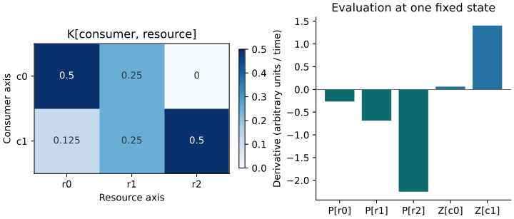
This synthetic example evaluates one state; it does not integrate a trajectory. Its binary-exact inputs are retained with the generated figure. The two consumer entries use different declared loss choices.

State	Value	Compiled derivative
P[r0]	1	-0.265625
P[r1]	2	-0.6875
P[r2]	4	-2.25
Z[c0]	0.5	0.0625
Z[c1]	1.5	1.40625

Vector PDF · Inputs and outputs

Conditional selection

np.where(condition, a, b) selects elementwise and dispatches through the state's array namespace. Conditions and branches can use shaped parameters, states and aliases. A condition such as linear[consumer] > 0 chooses the formula separately for each consumer.

Both branch expressions are evaluated. This is not lazy control flow: an inactive branch can still divide by zero, overflow or produce invalid gradients. Write expressions with valid numerical domains on both branches. Boolean parameters here choose between formulas; they do not create a stochastic event or change the reaction-network interpretation.

Lowering and cost

For a single unweighted, unfiltered reduction over one axis and one free output axis, the compiler recognizes a two-axis matrix multiplied by a one-axis vector or vector product. It emits namespace-native matmul, avoiding the broadcast matrix-vector temporary. Named axes supply the transpose when needed. More general layouts, weighted quadrature, filtered sums and repeated physical-axis forms retain the general reduction path.

Vectorized flat and PyTree evaluators cache generated expression functions at compile time. Each call binds fresh state and parameter values; it does not invoke eval for each alias or equation. State/parameter shape checks and namespace discovery still have per-call costs. Scalar fallback evaluation is unchanged, and small problems can still spend more time in dispatch than in arithmetic. No runtime speed ratio is guaranteed.

An optional warmed NumPy comparison records compilation separately from evaluation and checks the independent equations before timing:

OPENBLAS_NUM_THREADS=1 OMP_NUM_THREADS=1 uv run python -m \
  scripts.benchmark_named_kernels --sizes 4 16 128 256 512 1024

Large normalization cases can consume substantial time and memory. Start with the default smaller sweep when exploring a machine. These measurements are outside CI; CI checks numerical behavior and contraction structure without a wall-time threshold.