Trait-structured chemostat PDE

The chemostat_pde.py example couples a population density over a continuous trait coordinate to one well-mixed resource. It demonstrates non-uniform finite-volume geometry, implicit diffusion, nonlinear explicit coupling, and structured observables in one reproducible comparison.

Model and split

For population density n(theta, t) and resource S(t), the example solves

dn/dt = n g(theta, S) - D n + d d2n/dtheta2
dS/dt = D (S_in - S) - integral[n g(theta, S) w(theta) dtheta].

Growth combines Monod resource limitation with a Gaussian trait optimum. The positive uptake weight varies exponentially with trait and is scaled by the yield coefficient.

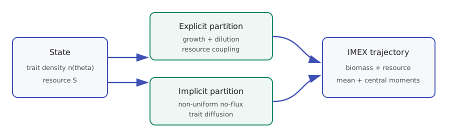
The split supplied to CoreSolver is:

Partition	Terms
implicit linear	no-flux trait diffusion
explicit nonlinear	growth, dilution, resource inflow, and consumption

imex-heun-tr treats the two partitions to second order. The implicit stage is assembled additively as L y = R y_n + explicit_increment; the right trapezoidal operator does not multiply the explicit increment.

The example does not clip stage states or project the result onto the positive orthant. Positivity in the canonical run is an observed numerical diagnostic, not an extra model operation.

Non-uniform finite volumes

build_trait_grid() calls generate_adaptive_grid() on the curvature of the initial Gaussian trait profile. More centers are placed where the initial profile bends rapidly, while the domain endpoints remain fixed.

For adjacent center spacings h_i, the integration weights are

q_0     = h_0
q_i     = (h_(i-1) + h_i) / 2
q_(N-1) = h_(N-2).

These are the same control-volume widths used by the non-uniform diffusion operator. With reflecting boundaries, q^T A = 0, so diffusion alone conserves total biomass.

Structured observables

At every output time the example records resource and five summaries of the trait distribution:

Observable	Discrete definition
biomass	I = sum_i q_i n_i
mean trait	rho = sum_i q_i n_i theta_i / I
variance	Sigma = sum_i q_i n_i (theta_i-rho)^2 / I
skewness	third central moment divided by Sigma^(3/2)
kurtosis	fourth central moment divided by Sigma^2

Kurtosis is the raw standardized fourth moment, not excess kurtosis.

Run and interpret the comparison

From a development checkout:

uv sync --dev
uv run python examples/chemostat_pde.py

The command writes examples/output/chemostat_pde/chemostat_summary.png and reports maximum state and biomass differences. The committed reference figure below uses the default 41-cell grid and 0.02-day time step.

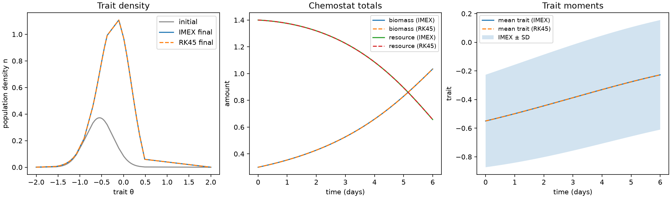
The panels compare initial and final trait densities, resource and total biomass, and the evolving mean trait with one standard deviation. Dashed lines come from SciPy RK45 applied to the same semi-discrete system with tight tolerances. This comparison isolates time integration: RK45 uses the identical grid, quadrature, reaction functions, diffusion matrix, and initial state.

The RK45 trajectory is a high-accuracy reference for this finite-dimensional discretization, not an exact solution of the continuous PDE. Grid convergence and time-step convergence remain separate checks.