Basic SIR Model

SIR model

Simulate data

We will use data simulated from a basic SIR model for 500 households. We will assume that all individuals start susceptible. The per day intra-household infection probability is 5% and the daily extra-household infection probability is 1%.

head(sir)

##   t part_id enroll state hh_size hh_id pcr igg
## 1 1       1      1     1       3     1   0   1
## 2 1       2      1     1       3     1   0   0
## 3 1       3      0     1       3     1   0   0
## 4 2       1      1     1       3     1   0   0
## 5 2       2      1     1       3     1   0   0
## 6 2       3      0     1       3     1   0   0

Model specification

In addition to the data, the user needs to specify the underlying model structure, which involves two components:

The infection process model which specifies the underlying compartmental model structure.
The observation process model which specifies the probability of observing a positive outcome given an individual is in each compartment of the infection process model.

Infection process model

The infection process model is built up from a series of user-defined transitions. There are two types of transitions: transmit() defines a transition that occurs as a result of infection (e.g. S>I) and progress() which defines a non-infection transition that occurs at a constant rate (e.g. I->R). For both functions, the user specifies a destination (e.g from = S) and source (e.g to = I) compartment. Additionally for progress() transitions, the user must enter a parameter for the transition rate. The name of this parameter is at the discretion of the user (e.g. gamma for recovery rate) and can be set to a specific numeric value of to NA if model should fit that parameter.

# Basic SIR, fit recovery rate
inf_process <- make_infection_model(transmit(from = "S", to = "I"),
                                    progress(from = "I", to = "R", gamma = NA))

Observation process model

The observation model is composed of a series of named vectors. Each vector corresponds to an observation type. Each entry in the vector is named for the corresponding compartment in the infection process model. The value is the probability of observing a positive observation given the individual is in the compartment.

In this example we have two observation types, one which is likely to be positive when a person is actively infectious (e.g. PCR test results) and the other which is more likely to be positive when the person is recovered and immune to infection (e.g. IgG antibody).

obs_process <- make_observation_model(
  pcr = c("S" = 0.05, "I" = 0.95, "R" = 0.05),
  igg = c("S" = 0.01, "I" = 0.01, "R" = 0.8)
)

Now we are ready to run the model!

# Note this is very computationally intensive so the block is not evaluated
# when knitting

## Inputs
# 1. Infection process model
# 2. Observation process model
# 3. Raw data
# 4. Covariates (optional)
# 5. Starting state probabilities

sir_res <- run_model(
  inf_model = inf_process,
  obs_model = obs_process,
  data = sir,
  init_probs = c(1 - 2 * 1e-10, 1e-10, 1e-10),
  stan_opts = stan_options(iter = 1000)
)

Now let’s look at the model results using the posterior package.

# The output from the model in the previous code chunk is available in the
# sir_res package data object

# Get summary statistics. Parameters are returned on the natural (model) scale,
# so no back-transformation is needed.
draws_sum <- summarise_draws(sir_res, "mean", "median", ~ quantile2(.x, probs = c(0.025, 0.975))) |>
  mutate(var_type = c(rep("Infection probability", 2), "Recovery rate"))

# "True" values from underlying simulation
draws_sum$true_value <- c(0.01, 0.05, 0.2)

draws_sum

## # A tibble: 3 × 7
##   variable    mean  median    q2.5  q97.5 var_type              true_value
##   <chr>      <dbl>   <dbl>   <dbl>  <dbl> <chr>                      <dbl>
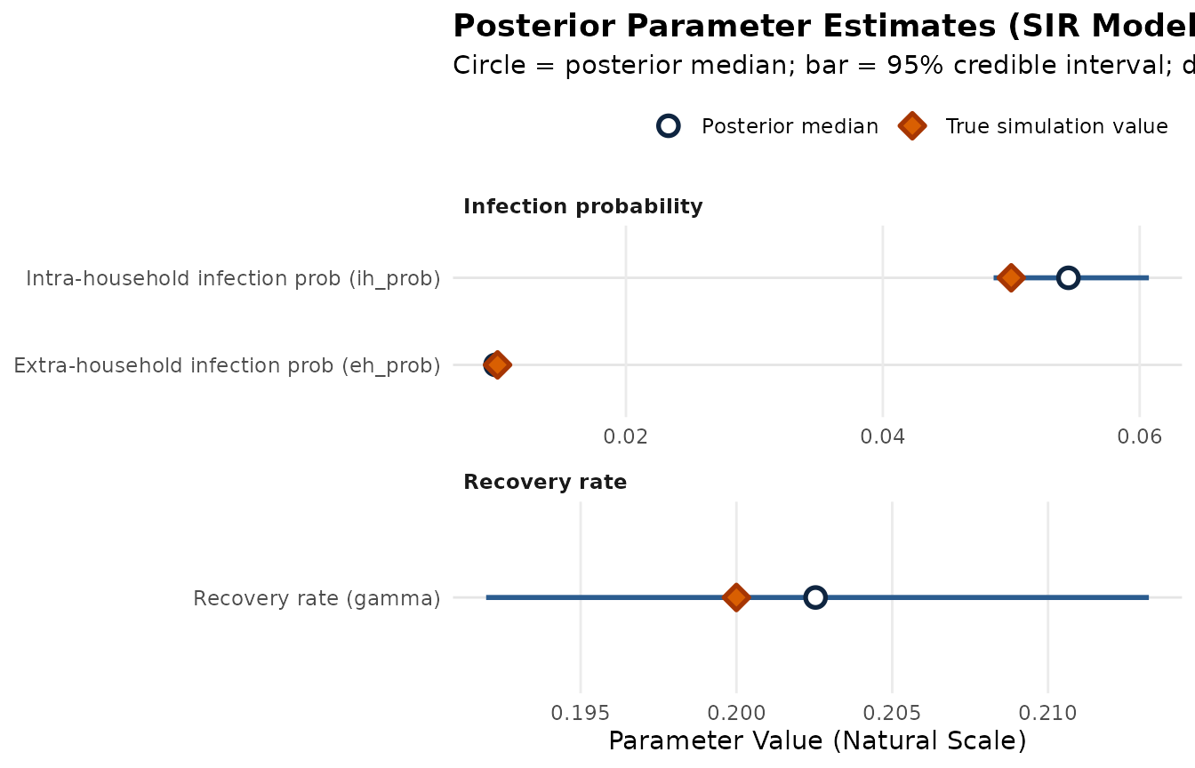
## 1 eh_prob  0.00984 0.00984 0.00911 0.0105 Infection probability       0.01
## 2 ih_prob  0.0545  0.0545  0.0486  0.0607 Infection probability       0.05
## 3 gamma    0.203   0.203   0.192   0.213  Recovery rate               0.2

We can also visualize the parameter estimates alongside the true simulation values:

draws_plot <- draws_sum |>
  mutate(
    label = factor(
      c("Extra-household infection prob (eh_prob)",
        "Intra-household infection prob (ih_prob)",
        "Recovery rate (gamma)"),
      levels = c("Extra-household infection prob (eh_prob)",
                 "Intra-household infection prob (ih_prob)",
                 "Recovery rate (gamma)")
    )
  )

ggplot(draws_plot, aes(y = label)) +
  geom_errorbar(aes(xmin = q2.5, xmax = q97.5), width = 0, color = "#2b5c8f", linewidth = 1) +
  geom_point(aes(x = median, fill = "Posterior median"), size = 3, shape = 21, color = "#0f2540", stroke = 1.4) +
  geom_point(aes(x = true_value, fill = "True simulation value"), size = 3, shape = 23, color = "#a63603", stroke = 1.4) +
  facet_wrap(~var_type, scales = "free", ncol = 1) +
  scale_fill_manual(
    name = "",
    values = c("Posterior median" = "#ffffff", "True simulation value" = "#d95f02"),
    guide = guide_legend(override.aes = list(
      shape = c(21, 23),
      color = c("#0f2540", "#a63603"),
      fill = c("#ffffff", "#d95f02")
    ))
  ) +
  labs(
    title = "Posterior Parameter Estimates (SIR Model)",
    subtitle = "Circle = posterior median; bar = 95% credible interval; diamond = true simulation value",
    x = "Parameter Value (Natural Scale)",
    y = NULL
  ) +
  theme_minimal() +
  theme(
    legend.position = "top",
    legend.justification = "right",
    panel.grid.minor = element_blank(),
    panel.grid.major.y = element_line(color = "grey90"),
    plot.title = element_text(face = "bold"),
    strip.text = element_text(face = "bold", hjust = 0)
  )

Add in covariates

We can add covariates on the intra- and extra-household infection risk by including the optional ih_cov and eh_cov arguments, respectively, in run_model().

# Simulated data from a basic SIR model for 500 households
head(sir_cov$observations)

# Run model with x1 and x2 as covariates
sir_cov_res <- run_model(
  inf_model = inf_process,
  obs_model = obs_process,
  data = sir_cov$observations,
  ih_cov = sir_cov$covariates,
  eh_cov = sir_cov$covariates,
  init_probs = c(1 - 2 * 1e-10, 1e-10, 1e-10),
  stan_opts = stan_options(iter = 1000)
)

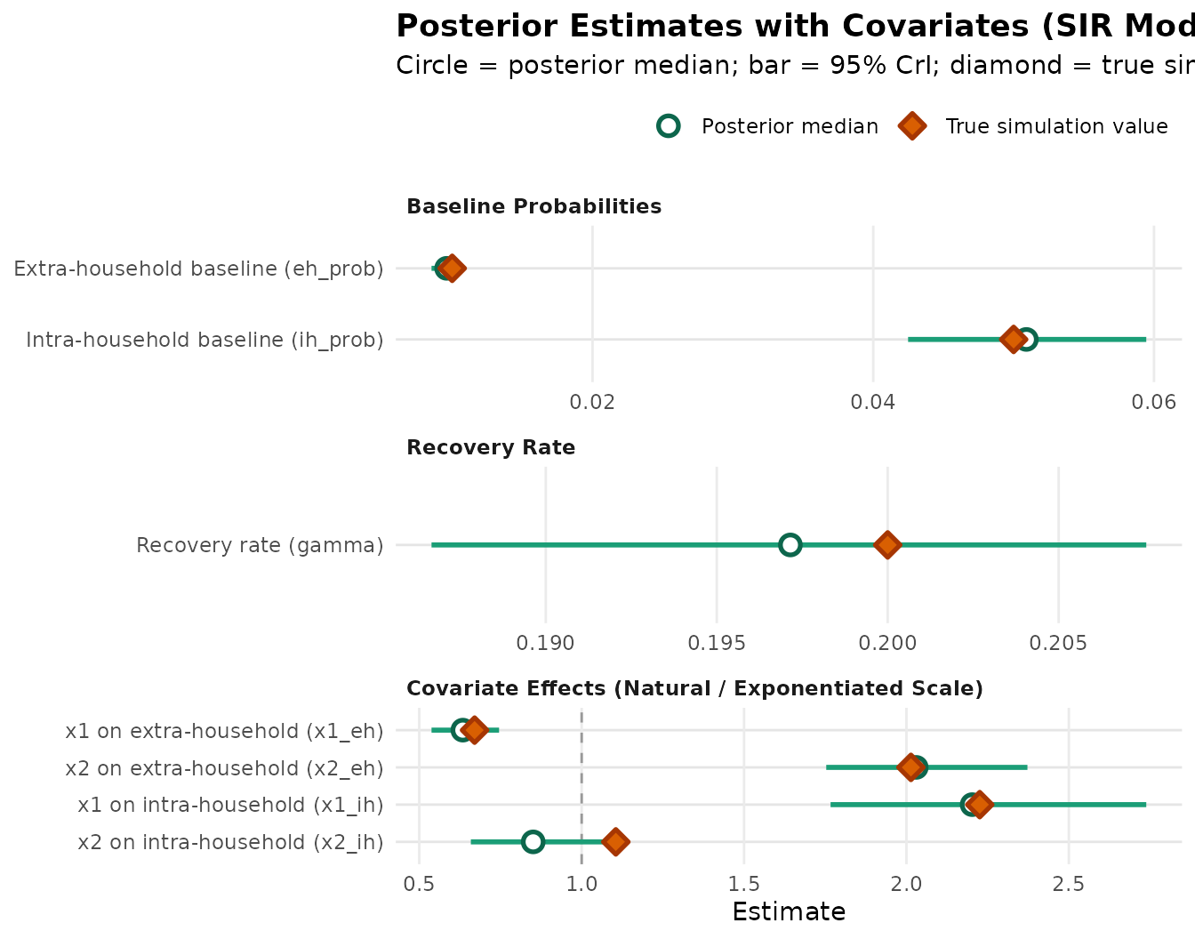
Let’s take a look at the results once more.

# The output from the model in the previous code chunk is available in the
# sir_cov_res package data object

# Get summary statistics. Infection probabilities and rates are returned on the
# natural (model) scale and coefficients on the natural (exponentiated) scale,
# so no back-transformation is needed.
draws_sum <- summarise_draws(sir_cov_res, "mean", "median",
                             ~ quantile2(.x, probs = c(0.025, 0.975))) |>
  mutate(var_type = c(rep("Infection probability", 2), "Recovery rate", rep("Coefficient", 4)))

# "True" values from underlying simulation
draws_sum$true_vals <- c(0.01, 0.05, 0.2, exp(-0.4), exp(0.7), exp(0.8), exp(0.1))

draws_sum

## # A tibble: 7 × 7
##   variable    mean  median    q2.5  q97.5 var_type              true_vals
##   <chr>      <dbl>   <dbl>   <dbl>  <dbl> <chr>                     <dbl>
## 1 eh_prob  0.00961 0.00960 0.00853 0.0108 Infection probability     0.01 
## 2 ih_prob  0.0509  0.0509  0.0425  0.0594 Infection probability     0.05 
## 3 gamma    0.197   0.197   0.187   0.208  Recovery rate             0.2  
## 4 x1_eh    0.636   0.634   0.538   0.746  Coefficient               0.670
## 5 x2_eh    2.03    2.03    1.75    2.37   Coefficient               2.01 
## 6 x1_ih    2.22    2.20    1.77    2.74   Coefficient               2.23 
## 7 x2_ih    0.857   0.851   0.659   1.10   Coefficient               1.11

We can plot the baseline probabilities, recovery rate, and covariate effects on the natural (exponentiated) scale: