Forecast hospital census from forecasting hubs

Public health forecasting hubs (FluSight, COVIDhub, RSVhub) publish admission forecasts. Hospital operations plan around the census: the number of patients in hospital on a given day. censcast turns one into the other by convolving admissions with a length of stay (LOS) distribution:

$$\text{census}(t) \;=\; \sum_{d \ge 0} \text{admissions}(t - d) \cdot P(\text{LOS} > d).$$

library(censcast)
library(dplyr)
library(purrr)
library(ggplot2)

What the hubverse gives you

Two tibbles in standard hubverse shape, both shipped with the package as toy data for this vignette:

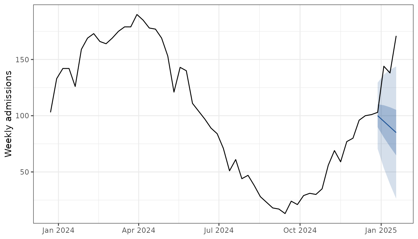
• admission_history: observed weekly admissions, as you would pull from a hub’s target time series (hubData::connect_target_timeseries()).
• admission_forecast: the next 4 weeks of admission quantile forecasts, as you would pull from a hub (hubData::connect_hub() |> collect_hub()).

Overlaying the two on one axis shows what a hub publishes: history in black, forecast fan in blue.

plot_fan(admission_forecast, truth = admission_history) +
  labs(y = "Weekly admissions")

censcast gives two ways to turn this into a census forecast, depending on whether you have past census data.

1. With past census data: fit_los()

Hubs publish admissions truth, not census truth, so the census series has to come from your own records. The package ships a toy version, census_history, generated by convolving admission_history with a known LOS, so it pairs row for row with the admission series.

fit_los() recovers the LOS by deconvolving the paired admission and census time series:

fit <- fit_los(
  data = inner_join(
    admission_history |> select(target_end_date, admissions = observation),
    census_history |> select(target_end_date, census = observation),
    by = "target_end_date"
  ),
  family = "negbin",
  max_stay = 8
)
fit
#> <los_fit> family=negbin  mu=2, k=1.7  P(LOS>8) = 0.0134

plot(fit) shows the recovered survival curve:

plot(fit)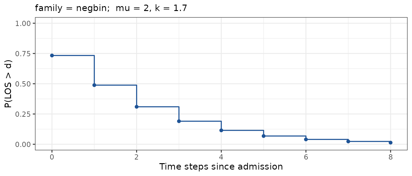

Drop the fit into fcast_census() to get a census forecast, then overlay the observed census to check the alignment:

census_fit <- fcast_census(admission_forecast, fit, admission_history)
plot_fan(census_fit, truth = census_history) +
  labs(y = "Weekly census")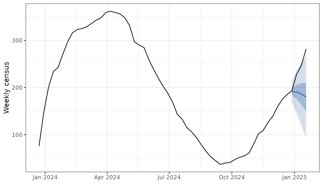

2. Without past census data: spec_los()

If no census data is available, set LOS from literature priors. Running several priors makes the assumption visible. Short stays put weight on recent admissions; long stays smooth across many weeks:

los_priors <- list(
  "short (mu=0.5w)" = spec_los("negbin", mu = 0.5, k = 1.7, max_stay = 8),
  "medium (mu=2w)" = spec_los("negbin", mu = 2, k = 1.7, max_stay = 8),
  "long (mu=4w)" = spec_los("negbin", mu = 4, k = 1.7, max_stay = 8)
)

census_priors <- imap(los_priors, \(s, name) {
  fcast_census(admission_forecast, s, admission_history) |>
    mutate(los = name)
}) |>
  bind_rows()

# Replicate truth across facets so each panel gets the black line.
truth_faceted <- imap(los_priors, \(s, name) {
  mutate(census_history, los = name)
}) |>
  bind_rows()

plot_fan(census_priors, truth = truth_faceted) +
  facet_wrap(~los, ncol = 1) +
  labs(y = "Weekly census")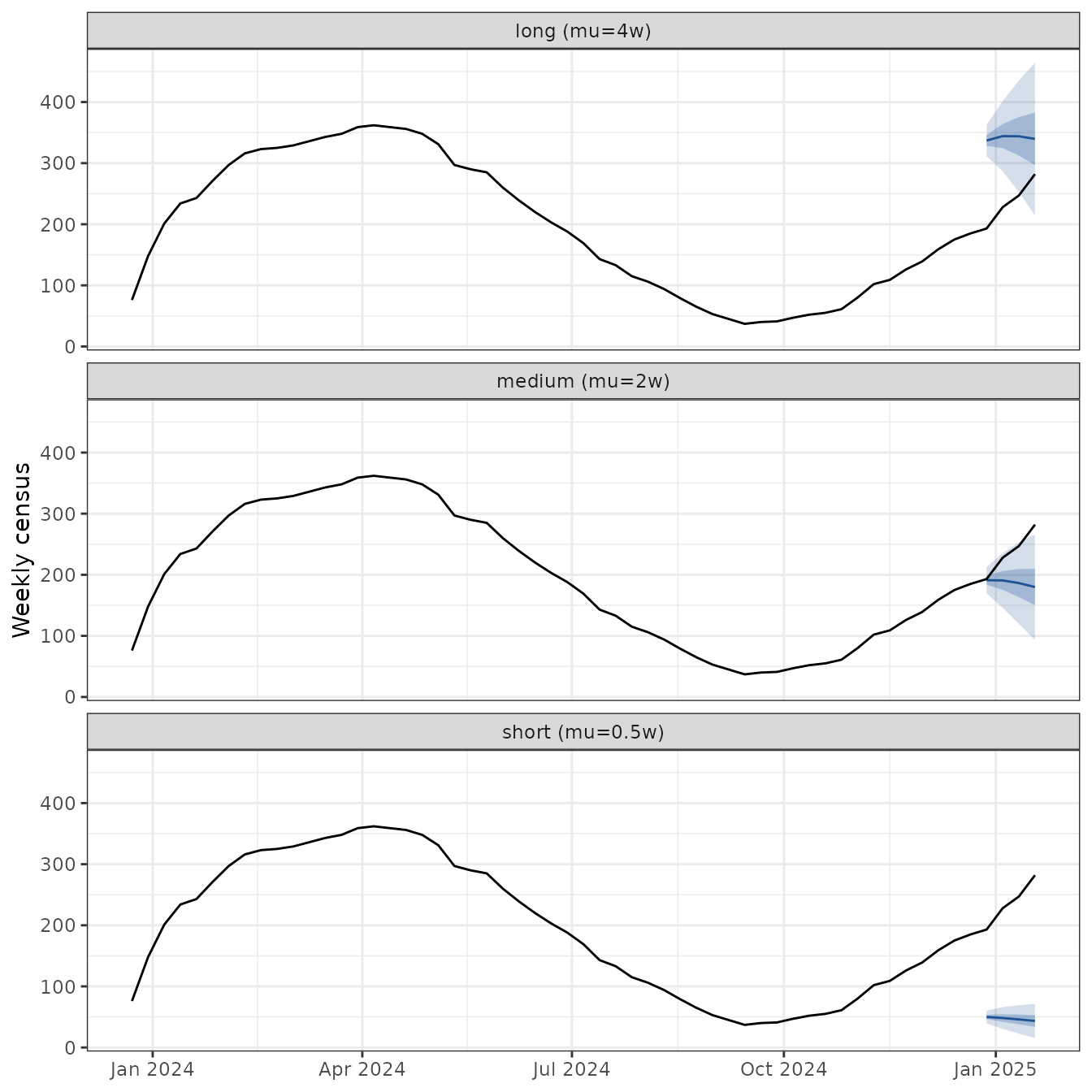

plot_fan() treats any unrecognised column as a trajectory grouper, so the user added los column needs no configuration.

3. Scoring

score_census() returns weighted interval score (WIS) per quantile via scoringutils. Pair each forecast with the truth and compare mean WIS across LOS priors:

imap(los_priors, \(s, name) {
  fcast_census(admission_forecast, s, admission_history) |>
    score_census(census_truth = census_history) |>
    mutate(los = name)
}) |>
  bind_rows() |>
  summarise(mean_wis = mean(wis), .by = los) |>
  arrange(mean_wis)
#>               los  mean_wis
#> 1  medium (mu=2w)  29.69379
#> 2    long (mu=4w)  76.89364
#> 3 short (mu=0.5w) 181.69018

The “medium” prior matches the LOS used to generate census_history (negbin(mu = 2, k = 1.7)), so it wins. In a real workflow, lean on fit_los() when census data exists and use spec_los() priors as a sensitivity check.

Plugging in a real hub

The toy datasets above are the only difference between this vignette and a production workflow. Swap them for live hub data:

library(hubData)

admission_forecast <- connect_hub(s3_bucket("cdcepi-flusight-forecast-hub")) |>
  dplyr::filter(
    target == "wk inc flu hosp",
    output_type == "quantile",
    model_id == "FluSight-ensemble"
  ) |>
  collect_hub()

admission_history <- connect_target_timeseries(
  s3_bucket("cdcepi-flusight-forecast-hub")
) |>
  dplyr::filter(target == "wk inc flu hosp") |>
  dplyr::collect()

census_history (or its real equivalent) you supply from your own records.

API

Function	Role
spec_los()	LOS survival vector from priors.
fit_los()	LOS survival vector fit from (admissions, census).
fcast_census()	Convolve admissions × LOS → census, hubverse shape in/out.
plot_fan()	Quantile fan chart, returns a ggplot.
score_census()	Score census forecast against truth via scoringutils.